|
|
|
CHAPTER 10: UNSTEADY GRADUALLY VARIED FLOW |
10.1 GOVERNING EQUATIONS
|
|
Three conservation principles are applicable in open-channel flow:
Conservation of mass, which could be either: (a) steady, or (b) unsteady,
Conservation of energy, which is steady (recall that energy is equal to the integral of all forces, excluding inertia,
in space, Eq. 2-15), andConservation of momentum, which is unsteady (recall that momentum is equal to the integral of the inertia force
in time, Eq. 2-27).
Steady gradually varied flow combines the statements of steady conservation of mass and conservation of energy (Chapter 7). Unsteady gradually varied flow combines the statements of unsteady conservation of mass and conservation of momentum (Table 10-1). Thus, unsteady gradually varied flow differs from steady gradually varied flow in its description of the temporal variation of the flow variables (discharge, stage, flow depth, mean velocity, and so on).
In practice, steady gradually varied flow is simply referred to as "gradually varied flow" (GVF), while unsteady gradually varied flow is commonly referred to as "unsteady flow" (UF).
| Table 10-1 Conservation laws and types of gradually varied flow. | |||
| Model | First equation: Conservation of mass, either → | Steady mass | Unsteady mass |
| Second equation: Conservation of → | Energy | Momentum | |
| Flow | Type (name) → | Steady GVF | Unsteady GVF |
| Commonly referred to as → | Gradually varied flow | Unsteady flow | |
| Treated in → | Chapter 7 | Chapter 10 (this chapter) | |
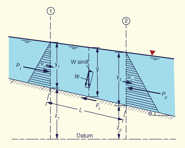
Figure 10-1 depicts the forces acting on a control volume. One body force and two surface forces are shown. The body force is the component of the gravitational force resolved along the direction of motion (W sin θ). The surface forces are: (1) the force due to the pressure gradient (due to the difference in flow depths), ΔP = P2 - P1, and (2) the force developed along the bottom boundary due to friction (Ff ). When these three forces are in equilibrium along the direction of motion, the flow is steady from the force standpoint. When the three forces are NOT in equilibrium along the direction of motion, the flow is unsteady and a fourth force arises (the inertia force) to produce a balance.
|
Governing equations
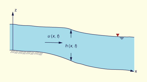
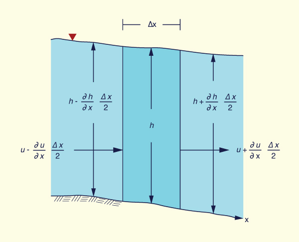
The derivation of the governing equations of unsteady flow (Fig. 10-2) (unsteady gradually varied flow) considers the statements of mass and momentum conservation in a control volume (Fig. 10-3).
|
|
The statement of conservation of mass is:
|
For a unit-width channel (Liggett, 1975):
|
∂u Δx ∂h Δx ∂u Δx ∂h Δx ∂h (u - ____ ____ ) (h - ____ ____ ) - (u + ____ ____ ) (h + ____ ____ ) = ____ Δx ∂x 2 ∂x 2 ∂x 2 ∂x 2 ∂t |
| (10-1) |
Simplifying, and neglecting second-order terms as Δx → 0:
|
∂h ∂h ∂u ____ + u ____ + h ____ = 0 ∂t ∂x ∂x | (10-2) |
|
∂h ∂ ____ + ____ (uh) = 0 ∂t ∂x | (10-3) |
Equation 10-3 is the unsteady conservation of mass equation, commonly referred to as the equation of continuity. However, its complete name is: the differential equation of water continuity.
For steady flow: ∂h/∂t = 0, and Eq. 10-3 reduces to: q = uh = constant. In general, for a channel of flow area A, the steady water continuity equation is: Q = uA = constant.
The statement of conservation of momentum is:
|
The momentum, per unit of channel width, is: ρ u (uh). Therefore, the net rate of momentum entering the control volume FΔ (force per unit of width) is:
|
∂ Δx ∂ Δx FΔ = ρ { u (u h) - ____ [ u (u h) ] ____ } - ρ { u (u h) + ____ [ u (u h) ] ____ } ∂x 2 ∂x 2 |
| (10-4) |
The forces acting on the control volume, resolved along the direction of motion, are: (1) gravitational force, (2) pressure-gradient force, and (3) frictional force (Fig. 10-1).
The gravitational force, per unit of width, is:
|
Fg = ρ g h Δx sin θ ≅ ρ g h Δx tan θ = ρ g h Δx So | (10-5) |
The pressure-gradient force, per unit of width, developed along the sides of the control volume, is:
|
h h 1 Fp = ∫ p dz = ρ g ∫ (h - z ) dz = = ____ ρ g h 2 0 0 2 | (10-6) |
The frictional force, per unit of width, developed along the channel bottom, resembles the gravitational force, but it is opposite in sign:
|
Ff = - ρ g h Δx Sf | (10-7) |
in which Sf = friction slope. [As an exception, for channels of adverse bottom slope, for which So < 0, the gravitational and frictional forces are of the same sign].
The size of the control volume, per unit of width, is:
|
∂ Fm = ____ (ρ u h) Δx ∂t | (10-8) |
The conservation of momentum is:
|
FΔ + Fg + Fp + Ff = Fm | (10-9) |
Replacing Eqs. 10-4 to 10-8 into Eq. 10-9:
|
∂ Δx ∂ Δx ρ { (u 2 h ) - ____ (u 2 h ) ____ } - ρ { (u 2 h ) + ____ (u 2 h ) ____ } + ρ g h Δx So ∂x 2 ∂x 2 |
|
1 ∂h 2 Δx ∂h 2 Δx + ____ ρ g [ (h 2 - _____ ____ ) - (h 2 + _____ ____ ) ] + ρ g h Δx Sf 2 ∂x 2 ∂x 2 |
|
∂ = ____ (ρ u h) Δx ∂t | (10-10) |
Simplifying Eq. 10-10:
|
∂ ∂ g ∂h 2 ____ (u h ) + ____ (u 2 h ) + ____ ______ = g h (So - Sf ) ∂t ∂x 2 ∂x | (10-11) |
Equation 10-11 is in conservation form. For certain applications, it must remain in this form. However, it is often expressed in reduced form, by operating on the derivatives:
|
∂u ∂h ∂ ∂u ∂h h ____ + u ____ + u ____ (u h ) + (u h ) ____ + g h ____ = g h (So - Sf ) ∂t ∂t ∂x ∂x ∂x |
| (10-12) |
The second and third terms of Eq. 10-12 have implicit in them the continuity equation (Eq. 10-3). Thus, Eq. 10-12 reduces to:
|
∂u ∂u ∂h ____ + u ____ + g ____ + g (Sf - So ) = 0 ∂t ∂x ∂x | (10-13) |
By dividing by g, Eq. 10-13 is expressed in slope units:
|
1 ∂u u ∂u ∂h ____ _____ + ____ _____ + _____ + (Sf - So ) = 0 g ∂t g ∂x ∂x | (10-14) |
Equation 10-14 is referred to as the equation of motion.
It is expressed in terms of slopes as follows:
|
Sa + Sc + Sp + Sf - So = 0 | (10-15) |
in which Sa = local acceleration slope, Sc = convective acceleration slope, Sp = pressure-gradient slope, Sf = friction slope, and So = bottom slope.
Wave types
Equation 10-15 indicates that the momentum balance is essentially a balance of slopes. In the general case, when all forces are present, all slopes are acting and the solution is the most general. In certain cases, however, one or more slopes may be reduced to zero, or assumed to be negligible (compared to the remaining slopes). This simplification gives rise to several types of waves, described in Table 10-2.
| Table 10-2 Types of waves in unsteady open-channel flow. | ||||||||
| No. | Wave type | Slopes | Common name | Applications | Sa
| Sc
| Sp
| Sf
| So
| 1
| Kinematic wave
|
|
|
| ✓
| ✓
| Kinematic wave
| Overland flow
|
|
| ✓
| ✓
| ✓
| Diffusion wave
| Flood routing
| 3
| Dynamic wave
| ✓
| ✓
| ✓
|
|
| Gravity | wave small canals 4
| Steady-dynamic wave
|
| ✓
| ✓
| ✓
| ✓
| Steady-dynamic wave
| Special cases
| 5
| Mixed | ✓
| ✓
| ✓
| ✓
| ✓
| Dynamic wave
| Dam-breach | |
|
Applicability of wave types
Kinematic waves [1] apply to overland flow, where the bottom slopes are steep, typically greater than So > 0.01. Diffusion waves [2] apply to flood routing in streams and rivers, with intermediate bottom slopes (0.01 > So > 0.0001). Dynamic waves [3] apply to the short waves of laboratory flumes and small canals. Steady-dynamic waves [4] apply to the few special cases where the neglect of the local acceleration term (Sa) is justified on practical grounds. In general, however, it is more accurate to neglect both Sa and Sc (i.e., a diffusion wave [2]) than just Sa (Ponce, 1990).
Mixed kinematic-dynamic waves [5]
apply to a sudden wave such as that originating in a dam breach, and may
also apply to channels
of very mild slope |
10.2 LINEAR SOLUTION
|
|
Equations 10-2 and 10-14 are the governing equations of continuity and motion, also referred to as the Saint-Venant equations (Saint-Venant, 1871). They are repeated here for convenience, as Eqs. 10-16 and 10-17, respectively.
|
∂h ∂h ∂u ____ + u ____ + h ____ = 0 ∂t ∂x ∂x | (10-16) |
|
1 ∂u u ∂u ∂h ____ _____ + ____ _____ + _____ + (Sf - So ) = 0 g ∂t g ∂x ∂x | (10-17) |
These equations constitute a set of two nonlinear (actually, quasilinear) partial differential equations, which when appropriately combined, result in a second-order partial differential equation of the hyperbolic type, featuring two solutions. To this date, there is no closed-form analytical solution of the set of Eqs. 10-16 and 10-17. An approximate solution may be obtained by linearizing the equation set and using the tools of linear stability analysis (Ponce and Simons, 1977).
The friction slope Sf is directly related to the bottom shear stress τ by the expression (similar to Eq. 6-16):
|
τ Sf = _____ γ h | (10-18) |
In the usual manner of stability calculations, Eqs. 10-16 and 10-17 must satisfy the unperturbed flow, for which u = uo , h = ho , and τ = τo . They must also satisfy the perturbed flow, for which u = uo + u' , h = ho + h' , and τ = τo + τ' . The superscript ' represents a small perturbation to the steady uniform flow. Thus, all quadratic terms in the fluctuating components may be negledted due to an order-of-magnitude reasoning.
Substitution of the perturbed variables in Eqs. 10-16, 10-17, and 10-18, yields, after linearization (Lighthill and Whitham, 1955):
|
∂h' ∂h' ∂u' ____ + uo ____ + ho ____ = 0 ∂t ∂x ∂x | (10-19) |
|
1 ∂u' uo ∂u' ∂h' τ' h' ____ _____ + ____ _____ + _____ + So ( _____ - _____ ) = 0 g ∂t g ∂x ∂x τo ho | (10-20) |
in which:
|
τo So = _____ γ ho | (10-21) |
The boundary shear stress τ can be related to the mean velocity u as follows (Eq. 5-3):
|
τ = f ρ u 2 | (10-22) |
in which the friction factor f is (Eq. 5-12):
| g f = ______ C 2 | (10-23) |
In view of Eq. 10-22, Eq. 10-20 is converted to:
|
1 ∂u' uo ∂u' ∂h' u' h' ____ _____ + ____ _____ + _____ + - So ( 2 _____ - _____ ) = 0 g ∂t g ∂x ∂x uo ho | (10-24) |
Small perturbation analysis
The solution for a small perturbation in the depth of flow is postulated in the following exponential form (Ponce and Simons, 1977):
|
h' ____ = h* e i (σ* x* - β* t* ) ho | (10-25) |
in which the subscript * indicates dimensionless variables, and i = (-1)1/2. The quantity σ* = dimensionless wavenumber, β* = dimensionless complex propagation factor, and x* and t* are dimensionless space and time coordinates, such that:
|
2 π σ* = ( _____ ) Lo L | (10-26) |
|
2 π Lo βR* = ( _____ ) _____ T uo | (10-27) |
|
x x* = _____ Lo | (10-28) |
|
uo t* = t _____ Lo | (10-29) |
and βI* is an amplitude propagation factor. The quantity Lo is the length of channel in which the uniform flow drops a head equal to its depth:
|
ho Lo = _____ So | (10-30) |
The depth disturbance is associated with a velocity disturbance of the form:
|
u' ____ = u* e i (σ* x* - β* t* ) uo | (10-31) |
The substitution of Eqs. 10-25 and 10-31 into Eqs. 10-19 and 10-24 yields the set:
|
σ* u* + (σ* - β* ) d* = 0 | (10-32) |
|
[ 2 + i Fo2 (σ* - β* ) ] u* + (i σ* - 1 ) d* = 0 | (10-33) |
in which
|
uo 2 Fo2 = ______ g ho | (10-34) |
Equations 10-32 and 10-33 constitute a homogeneous system of linear equations in the unknowns u* and h*. For the solution to be nontrivial, the determinant of the coefficient matrix must vanish. Therefore, the following relation holds:
|
i β* 2 Fo2 - i σ* 2 (1 - Fo2 ) + 3 σ* - 2 β* - 2 i σ* β* Fo2 = 0 | (10-35) |
Equation 10-35 is the characteristic equation governing the propagation of small amplitude water waves. Through algebraic manipulation, Eq. 10-35 reduces to:
|
Fo2 β* 2 - 2 (σ* Fo2 - i ) β* - [ σ* 2 (1 - Fo2 ) + 3 σ* i ] = 0 | (10-36) |
The solution of Eq. 10-36 is (Ponce and Simons, 1977):
|
1 β* = σ* ( 1 - i ζ ) + σ* [ ( ______ - ζ 2 ) + i ζ ] 1/2 Fo2 | (10-37) |
in which
|
1 ζ = _________ σ* Fo2 | (10-38) |
The equations for dimensionless celerity and attenuation for the primary and secondary waves are:
|
C + A c1* = 1 + ( _________ )1/2 2 | (10-39) |
|
B - E δ1 = - 2π _____________ | 1 + D | | (10-40) |
|
C + A c2* = 1 - ( _________ )1/2 2 | (10-41) |
|
B + E δ2 = - 2π _____________ | 1 - D | | (10-42) |
in which
|
1 A = ______ - ζ 2 Fo2 | (10-43) |
|
B = ζ | (10-44) |
|
1 C = [ ( ______ - ζ 2 ) 2 + ζ 2 ] 1/2 Fo2 | (10-45) |
|
C + A D = ( _________ )1/2 2 | (10-46) |
|
C - A E = ( _________ )1/2 2 | (10-47) |
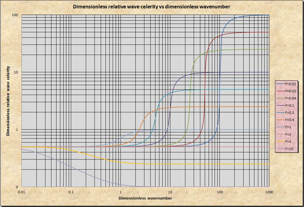
The dimensionless relative wave celerity is:
|
C + A cr* = ( _________ )1/2 = D 2 | (10-48) |
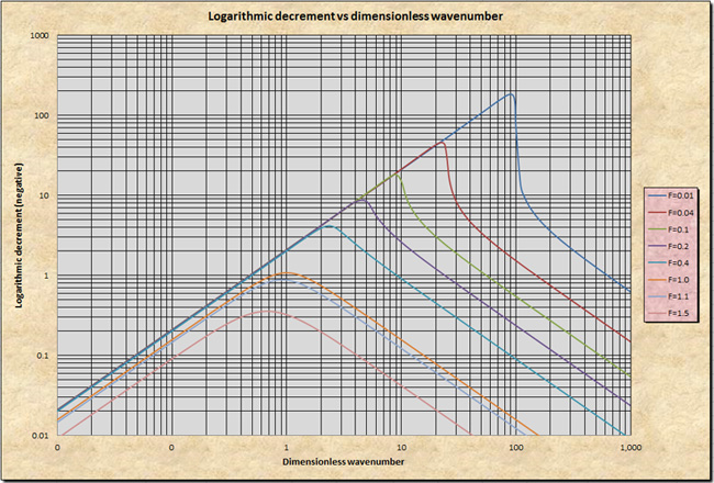
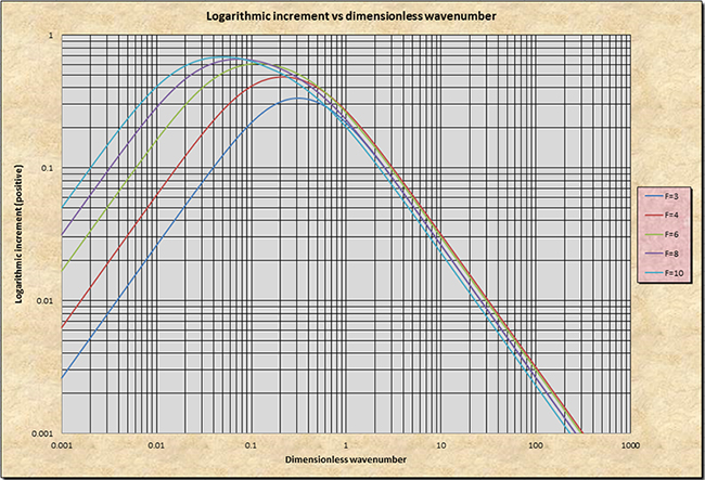
Figure 10-4 shows a plot of the dimensionless relative wave celerity cr* versus the dimensionless wavenumber σ*. Figure 10-5 shows a plot of the primary wave logarithmic decrement -δ1 versus the dimensionless wavenumber σ*, applicable for Froude numbers F < 2. Figure 10-6 shows a plot of the primary wave logarithmic increment +δ1 versus the dimensionless wavenumber σ*, applicable for Froude numbers F > 2. Based on these figures, the characteristics of shallow waves are described in the box below.
|
|
|
Shallow wave propagation in open-channel flow 1
1 See Ponce and Simons (1977) for a detailed treatment of shallow wave propagation in open-channel flow. |
10.3 KINEMATIC WAVES
|
|
A kinematic wave is an idealization (of gradually varied unsteady open-channel flow) that neglects both acceleration terms (local and convective) and the pressure-gradient term (Table 10-2). By neglecting these terms, the equation of motion (Eq. 10-14) is reduced to a statement of steady uniform flow:
|
Sf = So | (10-49) |
The unsteadiness of the phenomenon, however, is preserved through the time-varying term in the continuity equation (Eq. 10-3). The combination of Eqs. 10-3 and 10-49 gives rise to the kinematic wave equation.
Since q = uh, Eq. 10-3 may be expressed in terms of the unit-width discharge:
|
∂h ∂q ____ + ____ = 0 ∂t ∂x | (10-50) |
In terms of discharge Q, the continuity equation is:
|
∂A ∂Q _____ + _____ = 0 ∂t ∂x | (10-51) |
A statement of uniform flow (Eq. 10-49) may be properly represented by the discharge-area rating:
|
Q = α A β | (10-52) |
in which α and β are coefficient and exponent, respectively. The coefficient α varies as a function of type of friction, cross-sectional shape, and bottom slope. The exponent β varies as a function of type of friction and cross-sectional shape.
Assuming for the sake of simplicity that α and β are independent of A, Eq. 10-52 yields:
|
dQ _____ = α β A β - 1 dA | (10-53) |
|
dQ Q _____ = β ____ dA A | (10-54) |
|
dQ _____ = β V dA | (10-55) |
in which V = Q / A = mean velocity.
The kinematic wave equation is obtained by combining Eqs. 10-51 and 10-55 to yield:
|
∂Q ∂Q _____ + β V _____ = 0 ∂t ∂x | (10-56) |
In terms of unit-width discharge q :
|
∂q ∂q _____ + β V _____ = 0 ∂t ∂x | (10-57) |
Convective celerity
Equation 10-56 (or Eq. 10-57) is a first-order partial differential equation. It describes the convection of the quantity Q (or q) with the convective velocity or celerity ck, where ck is:
|
ck = β V | (10-58) |
Given Eq. 10-55, the convective velocity may also be expressed as:
|
dQ ck = _____ dA | (10-59) |
Given that dA = T dy (Eq. 3-11), where T = channel top width, and y = stage, the convective velocity may also be expressed as follows:
|
1 dQ ck = ____ _____ T dy | (10-60) |
Equation 10-60 was originally derived by Kleitz (1877) and was later discovered from actual field observations by Seddon (1900). It often referred to as the Kleitz-Seddon Law, or simply Seddon's Law. Equation 10-58 is used when β is known with certainty, Eq. 10-59 in theoretical formulations, and Eq. 10-60 in practical applications.
Since Eq. 10-56 is a first-order partial differential equation, it does not allow for wave diffusion (wave attenuation, or wave dissipation). Diffusion can only be obtained through the agency of a second-order term. Under the assumption of linearity (constant convective celerity), a kinematic wave will convect its discharge with no wave diffusion; that is, the discharge will retain its shape and remain constant in space and time upon propagation.
|
Absence of wave diffusion in the kinematic wave
The absence of wave diffusion can be further demonstrated by a mathematical argument. The total derivative for Q is:
Therefore:
The kinematic wave equation is repeated here:
Comparing Eq. 10-61 with Eq. 10-55, it follows that dQ/dt = 0, that is, Q remains constant in time for waves traveling with the convective celerity β V. |
Kinematic shock
When the linearity assumption is relaxed, the kinematic wave may change its shape by becoming either (a) steeper [Fig. 10-7 (a)], or (b) flatter [Fig. 10-7 (b)]. Whether a wave will steepen or flatten out will depend largely on the channel cross-sectional shape. Two asymptotic limits are recognized: (1) waves propagating in hydraulically wide channels, while (2) waves propagating in inherently stable channels (Chapter 1). In hydraulically wide channels, the waves will steepen, while in inherently stable channels, they will flatten out (Ponce and Windingland, 1985).
|
|
When allowed to proceed unchecked, the steepening will eventually result in a kinematic wave becoming a kinematic shock. Thus, a kinematic shock is an unsteady open-channel flow feature intrinsically related to the kinematic wave: A wave must be kinematic before it can develop into a kinematic shock (Lighthill and Whitham, 1955). Kibler and Woolhiser (1970) sought to clarify the occurrence of kinematic shock phenomena by stating:
|
Thus, the kinematic shock is real but rare in the physical world, where spatial irregularities manifest themselves as diffusion, with the net effect of arresting shock development. On the other hand, the computational world is likely to be much more regular, thereby inhibiting diffusion and promoting "numerical" shock development.
Kinematic wave celerity
The relative kinematic wave celerity, ie., the kinematic wave celerity taken relative to the flow velocity, is:
|
crk = (β - 1 ) V | (10-63) |
Furthermore, the dimensionless relative kinematic wave celerity is:
|
crk cdrk = _____ = β - 1 V | (10-64) |
According to Eq. 1-11, the relative dimensionless kinematic wave celerity is:
|
V cdrk = β - 1 = ____ F | (10-65) |
Thus, for V = 1, i.e., for neutrally stable flow, the Froude number is:
|
1 1 Fns = _______ = _______ β - 1 cdrk | (10-66) |
Table 10-3 shows the variation of: (a) the exponent β, (b) the dimensionless relative kinematic wave celerity cdrk, and (c) the neutral-stability Froude number, with selected types of friction and cross-sectional shape.
| Table 10-3 Variation of β as a function of type of friction and cross-sectional shape. | [1] | [2] | [3] | [4] | [5] | [6] |
| β | 24 β | Type of friction | Cross-sectional shape | cdrk | Fns |
| 3 | 72 | Laminar | Hydraulically wide | 2 | 1/2 |
| 8/3 | 64 | Mixed laminar-turbulent (25% turbulent Manning) | Hydraulically wide | 5/3 | 3/5 |
| 21/8 | 63 | Mixed laminar-turbulent (25% turbulent Chezy) | Hydraulically wide | 13/8 | 8/13 |
| 7/3 | 56 | Mixed laminar-turbulent (50% turbulent Manning) | Hydraulically wide | 4/3 | 3/4 |
| 9/4 | 54 | Mixed laminar-turbulent (50% turbulent Chezy) | Hydraulically wide | 5/4 | 4/5 |
| 2 | 48 | Mixed laminar-turbulent (75% turbulent Manning) | Hydraulically wide | 1 | 1 |
| 15/8 | 45 | Mixed laminar-turbulent (75% turbulent Chezy) | Hydraulically wide | 7/8 | 8/7 |
| 5/3 | 40 | Turbulent Manning | Hydraulically wide | 2/3 | 3/2 |
| 3/2 | 36 | Turbulent Chezy | Hydraulically wide | 1/2 | 2 |
| 4/3 | 32 | Turbulent Manning | Triangular | 1/3 | 3 |
| 5/4 | 30 | Turbulent Chezy | Triangular | 1/4 | 4 |
| 1 | 24 | Any | Inherently stable | 0 | ∞ |
The following conclusions can be drawn from Table 10-3:
The value of the rating exponent varies from as high as β = 3 for laminar flow in a hydraulically wide channel, to as low as
β = 1 for an inherently stable channel.The value of the dimensionless relative kinematic wave celerity varies from as high as cdrk = 2 for laminar flow in a hydraulically wide channel, to as low as cdrk = 0 for an inherently stable channel.
The Froude number for neutral stability varies from as low as Fns = 0.5 for laminar flow in a hydraulically wide channel (i.e., laminar overland flow), to as high as Fns = ∞ for an inherently stable channel under any type of friction (though usually turbulent).
The turbulent Chezy hydraulically wide dimensionless relative kinematic wave celerity is
cdrk = 0.5, confirming the results shown on (the left side of) Fig. 10-5. Thus, kinematic waves feature long wavelengths L and correspondingly "short" dimensionless wavenumbers σ* .The turbulent Manning hydraulically wide dimensionless relative kinematic wave celerity is
cdrk = 2/3, i.e., the Manning value exceeds the Chezy value by 1/6.
Note that the value of β may be less than 1 for cases other than those shown in Table 10-3; for example, when
the cross section does not grow monotonically with stage, as in circular culvert flow.
Also, note that since the Froude number has an upper limit (corresponding to a realistically achievable lower limit on the bottom friction),
the value Fns = ∞ is of limited practical value. If the maximum attainable Froude number is conservatively assumed to be
In summary, kinematic waves have the following properties:
Kinematic waves travel with dimensionless relative wave celerity equal to 0.5, under Chezy friction; under Manning friction, the value is 2/3.
Kinematic waves do not attenuate, but they can undergo changes in shape due to nonlinearities; in extreme cases in hydraulically wide channels, the kinematic wave may steepen to the point where it becomes a kinematic shock.
|
A word of caution regarding kinematic wave modeling 1
Despite the fact that wave attenuation is disavowed by kinematic wave theory, certain numerical solutions of Eq. 10-56 do exhibit a distinct attenuation. Cunge (1969) traced this apparent contradiction to the fact that numerical solutions, by virtue of their discrete grid size, introduce an error which expresses itself as numerical diffusion. As the grid is refined, the numerical effect decreases; however, a finite numerical grid (and all numerical grids are finite) will always have a residual error. The dilemma is resolved by making the numerical diffusion simulate the physical diffusion, if any, of the physical problem. This procedure is embodied in the Muskingum-Cunge method of flood routing, described in Section 10.6. 1 See Ponce (1991) for a detailed treatment of the controversy regarding kinematic waves. |
Kinematic wave rating
Kinematic waves are based on a single-valued discharge-area rating, Eq. 10-51. Thus, a kinematic wave rating is single-valued, exhibiting a one-to-one correspondence between (a) discharge, and (b) flow area, depth, or stage. A kinematic wave rating is calculated by using a uniform flow formula such as Manning or Chezy, for a range of (a) flow depths, in artificial channels, or (b) flow stages, in natural channels.
Applicability of kinematic waves
A kinematic wave is a simplified type of wave, wherein three terms in the equation of motion (Table 10-2) have been either neglected or assumed to be too small to be of any practical significance. Thus, the kinematic wave does not apply to the general case. Its use is recommended for cases where the flow unsteadiness is relatively small. In practice, a kinematic wave will apply provided the following dimensionless inequality is satisfied (Ponce, 1989; Ponce, 2014):
|
tr
So Vo
___________ ≥ 85 do | (10-67) |
in which tr = time-of-rise of the hydrograph, So = bottom slope, Vo = average flow velocity, and do = average flow depth.
10.4 DIFFUSION WAVES
|
|
A diffusion wave is an idealization that neglects both acceleration terms in the equation of motion (Table 10-2). By neglecting these terms, Eq. 10-14 is reduced to the following statement:
|
∂h Sf = So - _____ ∂x | (10-68) |
The unsteadiness of the phenomenon, however, is preserved through the time-varying term in the continuity equation (Eq. 10-3). The combination of Eqs. 10-3 and 10-68 gives rise to the diffusion wave equation.
The kinematic wave equation was derived by using a statement of steady uniform flow in lieu of the equation of motion (Section 10.4). In deriving the diffusion wave equation, a statement of steady nonuniform flow (friction slope is equal to water-surface slope) is used instead (Fig. 10-8). In this case, the discharge-area rating, using the Manning formula in SI Units (Eq. 5-17), is:
|
1 dh Q = ___ A R 2/3 (So - ____ ) 1/2 n dx | (10-69) |
in which the term within parentheses (...) is the water-surface slope Sw.
Figure 10-8 Diffusion wave assumption. |
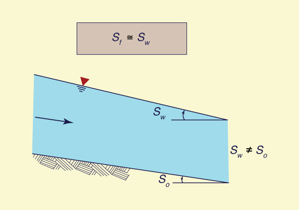
The difference between kinematic and diffusion waves lies in the pressure-gradient term (dh/dx). When this term is included in the formulation, the resulting equation is of second order and, therefore, it is able to simulate diffusion. Lighthill and Whitham (1955) referred to this situation as the "diffusion of kinematic waves," i.e., a type of kinematic wave, still with no inertia in its formulation, that is nevertheless able to diffuse.
To derive the diffusion wave equation, Eq. 10-51 is repeated here in a slightly different form:
|
∂Q ∂A _____ + _____ = 0 ∂x ∂t | (10-70) |
Equation 10-69 is expressed in a more convenient form (Cunge, 1969):
|
dh m Q 2 = So - ____ dx | (10-71) |
in which m is the reciprocal of the square of the channel conveyance K (Eq. 5-34), repeated here for convenience:
|
1 K = ___ A R 2/3 n | (5-34) |
With dA = T dh, in which T = top width, Eq. 10-71 changes to:
|
1 dA _____ ______ + m Q 2 - So = 0 T dx | (10-72) |
Equations 10-70 and 10-72 constitute a set of two partial differential equations describing diffusion waves. These equations can be combined into one equation with Q as dependent variable. However, it is first necessary to linearize the equations around reference flow values. For simplicity, a constant top width is assumed (i.e., a wide channel assumption).
The linearization of Eqs. 10-70 and 10-72 is accomplished by small perturbation theory (Cunge, 1969). The variables Q, A, and m can be expressed in terms of the sum of a reference value (with subscript o) and a small perturbation to the reference value (with superscript ' ): Q = Qo + Q' ; A = Ao + A' ; m = mo + m'. Substituting these into Eqs. 10-70 and 10-72, neglecting squared perturbations and subtracting the reference flow, leads to:
|
∂Q' ∂A' ____ + ____ = 0 ∂x ∂t | (10-73) |
and
|
1 ∂A' _____ ______ + Qo2 m' + 2 mo Qo Q' = 0 T ∂x | (10-74) |
Differentiating Eq. 10-73 with respect to x and Eq. 10-74 with respect to t gives:
|
∂2Q' ∂2A' ______ + _______ = 0 ∂x 2 ∂x ∂t | (10-75) |
|
1 ∂2A' ∂m' ∂Q' _____ _________ + Qo2 _____ + 2 mo Qo ______ = 0 T ∂x ∂t ∂t ∂t | (10-76) |
Using the chain rule and Eq. 10-73 yields:
|
∂m' ∂m' ∂A' ∂m' ∂Q' _____ = _______ _______ = - ______ ______ ∂t ∂A' ∂t ∂A' ∂x | (10-77) |
Combining Eq. 10-76 with Eq. 10-77:
|
1 ∂2A' ∂m' ∂Q' ∂Q' _____ ________ - Qo2 ______ ______ + 2 mo Qo ______ = 0 T ∂x ∂t ∂A' ∂x ∂t | (10-78) |
Combining Eqs. 10-75 and 10-78 and rearranging terms, yields:
|
∂Q' Qo ∂m' ∂Q' 1 ∂Q'2 ______ - _______ ______ ______ = _____________ _______ ∂t 2 mo ∂A' ∂x 2 T mo Qo ∂x2 | (10-79) |
By definition: mQ 2 = Sf (Eq. 10-70). Therefore:
|
∂Q' ∂Q Qo _____ = _______ = - _______ ∂m' ∂m 2 mo | (10-80) |
and also
|
So mo Qo = ______ Qo | (10-81) |
Substituting Eqs. 10-80 and 10-81 into Eq. 10-79, using the chain rule, and dropping the superscripts for simplicity, the following equation is obtained:
|
∂Q ∂Q ∂Q Qo ∂2Q ______ + ( ______ ) ______ = ( _________ ) _______ ∂t ∂A ∂x 2 T So ∂x2 | (10-82) |
The left side of Eq. 10-82 is recognized as the kinematic wave equation, with ∂Q/∂A as the kinematic wave celerity.
The right side is a second-order (partial differential) term that accounts for the physical diffusion effect.
The coefficient of the second-order term has the units of diffusivity
The hydraulic diffusivity, a characteristic of the flow and channel, is defined as follows:
|
Qo qo νh = _________ = _______ 2 T So 2 So | (10-83) |
in which qo = Qo /T is the reference discharge per unit of channel width. From Eq. 10-83, it is concluded that the hydraulic diffusivity is small for steep bottom slopes (e.g., those of mountain streams), and large for mild bottom slopes (e.g., those of large rivers near their mouths).
Equation 10-82 describes the movement of flood waves in a better way than Eq. 10-50. While it falls short from describing the full inertial effects, it does physically account for wave attenuation.
Equation 10-82 is a second-order parabolic partial differential equation. It can be solved analytically, leading to the diffusion analogy solution for flood waves (Hayami, 1951), or numerically with the aid of a numerical scheme for parabolic equations. An alternative approach is to match the hydraulic diffusivity (Eq. 10-83) with the numerical diffusion coefficient of the Muskingum flood routing method (Section 10.5). This approach is the basis of the Muskingum-Cunge method (Section 10.6).
Diffusion wave rating
Diffusion waves are not based on a single-valued discharge-area rating. Thus, a diffusion wave rating is not single-valued, exhibiting a loop. In general, however, the loop is relatively small and may be neglected on practical grounds. A kinematic wave rating may be used as an approximation in diffusion wave routing.
Diffusion wave celerity
According to Eq. 10-82, the diffusion wave celerity should be the same as the kinematic wave celerity (Ponce and Simons, 1977). However, diffusion waves attenuate; therefore, the actual discharge-area rating is not exactly single-valued. In practice, the difusion wave celerity equals the kinematic wave celerity only as an approximation.
Applicability of diffusion waves
A diffusion wave is a simplified type of wave, wherein two terms in the equation of motion (Table 10-2) have been either neglected or assumed to be too small to be of any practical significance. Thus, while the diffusion wave applies for a wider range of cases than the kinematic wave, it is still not suited to the general case. Its use is recommended for cases where the flow unsteadiness is small to medium size (where the wave remains within 30% of its original strength, within one period of propagation). A diffusion wave will apply provided the following dimensionless inequality is satisfied (Ponce, 1989; Ponce, 2014):
|
g
tr So ( ____ )1/2 ≥ 15 do | (10-84) |
in which tr = time-of-rise of the hydrograph, So = bottom slope, g = gravitational acceleration, and do = average flow depth.
Diffusion waves apply to problems of flood wave propagation (see Hayami's diffusion analogy of flood waves in the box below). While kinematic waves apply to flood waves that do not diffuse, diffusion waves apply to flood waves that attenuate appreciably. Where the diffusion wave fails to account for the wave propagation, only the mixed kinematic-dynamic wave (read "dynamic wave", Table 10-2) is able to solve the problem correctly. In practice, however, diffusion waves apply to a wide range of flood propagation problems.
|
Hayami's diffusion analogy of flood waves
In 1951, Hayami published a paper entitled "On the propagation of flood waves." In it, he argued that flood waves could be modeled with a convection-diffusion equation similar to Eq. 10-82. To put it in Hayami's words:
|
Dynamic hydraulic diffusivity
The hydraulic diffusivity (Eq. 10-83) is a fundamental property of diffusion waves. It states that the coefficient of diffusion is directly proportional to the unit-width discharge and inversely proportional to the channel slope. This conclusion ia applicable to diffusion waves, which are governed by the convection-diffusion equation represented by Eq. 10-82.
Using concepts of linear theory, Dooge (1973) has developed a convection-diffusion equation using the complete equation of motion. Dooge's approach extends
the concept of diffusion wave to the realm of dynamic waves (Table 10-2). When all terms are included in the
formulation, the hydraulic diffusivity is essentially a dynamic hydraulic diffusivity, expressed, for hydraulically wide channels, as follows:
|
qo F 2 νhF = _______ ( 1 - ______ ) 2 So 4 | (10-85) |
Ponce (1991) has expressed the dynamic hydraulic diffusivity in terms of the Vedernikov number, as follows:
|
qo νhV = _______ ( 1 - V 2 ) 2 So | (10-86) |
Unlike Eq. 10-85, Eq. 10-86 is not limited to hydraulically wide channels, being applicable to channels of any cross-sectional shape.
Equation 10-86 is altogether better than Eq. 10-83. They are equivalent only if V = 0, i.e., for very small Froude-number flows. For V = 1, using Eq. 10-86, the hydraulic diffusivity vanishes, while this is not the case for Eq. 10-83, for which the hydraulic diffusivity remains finite.
10.5 MUSKINGUM METHOD
|
|
The Muskingum method of flood routing was developed in connection with the design of flood protection schemes in the Muskingum River Basin, Ohio (Fig. 10-10) (McCarthy, 1938). It is the most widely used method of flood routing, with numerous applications in the United States and throughout the world.
Figure 10-10 The Muskingum river near Marietta, Ohio. |
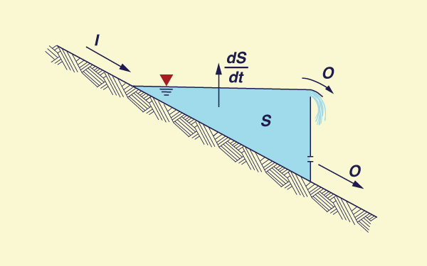
The method is based on the differential equation of storage (Fig. 10-11):
|
dS I - O = _____ dt | (10-87) |
in which I = inflow, O = outflow, and S = storage.
Figure 10-11 Definition sketch for inflow, outflow, and storage in a reservoir. |
In an ideal channel, storage is a function of inflow and outflow. This is in constrast with an ideal reservoir, in which storage is solely a function of outflow. In the Muskingum method, storage is a linear function of inflow and outflow:
| S = K [ X I + ( 1 - X ) O ] | (10-88) |
in which S = storage volume; I = inflow; O = outflow; K = a time constant or storage coefficient; and
To derive the Muskingum routing equation, Eq. 10-87 is discretized on the x-t plane (Fig. 10-12), to yield:
|
I1 + I2 O1 + O2 S2 - S1 __________ - ___________ = ___________ 2 2 Δt | (10-89) |
Figure 10-12 Discretization on the x-t plane. |
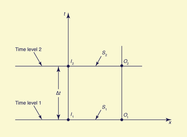
Equation 10-88 is expressed at time levels 1 and 2:
| S1 = K [ X I1 + ( 1 - X ) O1 ] | (10-90) |
| S2 = K [ X I2 + ( 1 - X ) O2 ] | (10-91) |
Substituting Eqs. 10-90 and 10-91 into Eq. 10-89 and solving for O2 yields:
| O2 = C0 I2 + C1 I1 + C2 I1 | (10-92) |
in which C0, C1 and C2 are routing coefficients defined in terms of Δt, K, and X as follows:
|
( Δt / K ) - 2X C0 = _______________________ 2(1 - X) + ( Δt / K ) | (10-93a) |
|
( Δt / K ) + 2X C1 = _______________________ 2(1 - X) + ( Δt / K ) | (10-93b) |
|
2(1 - X) - ( Δt / K ) C2 = _______________________ 2(1 - X) + ( Δt / K ) | (10-93c) |
Since C0 + C1 + C2 = 1, the routing coefficients may be interpreted as weighting coefficients.
Given an inflow hydrograph, an initial flow condition, a chosen time interval Δt, and routing parameters X and K, the routing coefficients can be calculated with Eq. 10-93, and the outflow hydrograph with Eq. 10-92. The routing parameters K and K are related to flow and channel characteristics, K being interpreted as the travel time of the flood wave from upstream end to downstream end of the channel reach. Therefore, K accounts for the translation portion of the routing (Fig. 10-12).
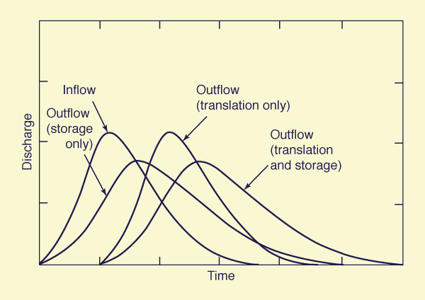
The parameter X accounts for the storage portion of the routing. For a given flood event, there is a value of X for which the storage in the calculated outflow hydrograph matches that of the measured outflow hydrograph. The effect of storage is to reduce the peak flow and spread the hydrograph in time (Fig. 10-13). Therefore, it is often used interchangeably with the terms diffusion and peak attenuation.
Figure 10-13 Translation and storage processes in stream channel routing. |
The routing parameter K is a function of channel reach length and flood wave speed; conversely, the parameter X is a function of the flow and channel characteristics that cause runoff diffusion. In the Muskingum method, X is interpreted as a weighting factor and restricted in the range 0 ≤ X ≤ 0.5. Values of X greater than 0.5 produce hydrograph amplification (i.e., negative diffusion), which does not correspond with reality (under the Froude numbers applicable to flood flows). With K = Δt and X = 0.5, flow conditions are such that the outflow hydrograph retains the same shape as the inflow hydrograph, but it is translated downstream a time equal to K. For X = 0, Muskingum routing reduces to linear reservoir routing.
In the Muskingum method, the parameters K and X are determined by calibration using streamflow records. Simultaneous inflow-outflow discharge measurements for a given channel reach are coupled with a trial-and-error procedure, leading to the determination of K and X (see Example 10-1). The procedure is time-consuming and lacks predictive capability. Values of K and X determined in this way are valid only for the given reach and flood event used in the calibration. Extrapolation to other reaches or to other flood events (of different magnitude) within the same reach is usually unwarranted.
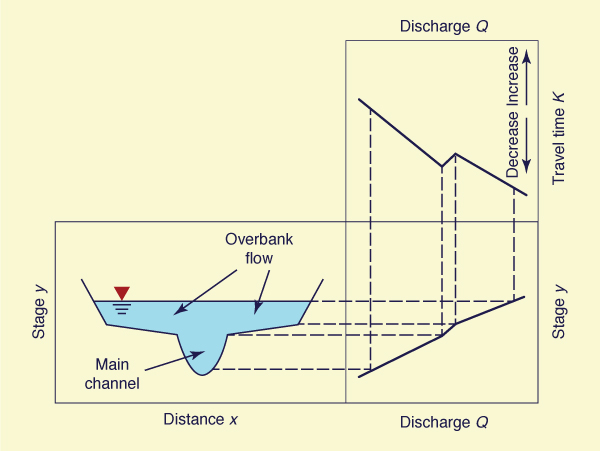
When sufficient data are available, a calibration can be performed for several flood events, each of different magnitude, to cover a wide range of flood levels. In this way, the variation of K and X as a function of flood level can be ascertained. In practice, K is more sensitive to flood level than X. A sketch of the variation of K with stage and discharge is shown in Fig. 10-14.
Figure 10-14 Sketch of travel time as a function of discharge and stage. |
Example 10-1.
An inflow hydrograph to a channel reach is shown in Col. 2 of Table 10-4.
Assume baseflow is 352 m3/s.
Using the Muskingum method, route this hydrograph through a channel reach with K = 2 d and X = 0.1 to calculate an outflow hydrograph.
First, it is necessary to select a time interval Δt.
In this case, it is convenient to choose Δt = 1 d.
As with reservoir routing, the ratio of time-to-peak to time interval
(tp /Δt ) should be greater than or equal to 5.
In addition, the chosen time interval should be such that the routing coefficients remain positive.
With Δt = 1 d, K = 2 d, and X = 0.1, the routing coefficients (Eq. 10-93) are: C0 = 0.1304; C1 = 0.3044; and C2 = 0.5652.
It is verified that C0 + C1 + C2 = 1.
The routing calculations are shown in Table 10-4.
Column 1 shows the time in days.
Column 2 shows the inflow hydrograph ordinates in cubic meters per second.
Columns 3-5 show the partial flows.
Following Eq. 10-91, Cols. 3-5 are summed to obtain Col. 6, the outflow hydrograph ordinates in cubic meters per second.
To explain the procedure briefly, the outflow at the start (day 0) is assumed to be equal to the inflow at the start: 352 m3/s. The inflow at day 1 multiplied by C0 is entered in Col. 3, day 1: 76.6 m3/s.
The inflow at day 0 multiplied by C1 is entered in Col. 4, day
1: 107.1 m3/s.
The outflow at day 0 multiplied by C2 is entered in Col. 5, day 1: 199 m3/s.
Columns 3-5 of day 1 are summed to obtain Col. 6 of day 1: 76.6 + 107.1 + 199.0 = 382.7 m3/s.
The calculations proceed in a recursive manner until all outflows in Col. 6 have been obtained.
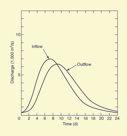
Inflow and outflow hydrographs are plotted in Fig. 10-15.
The outflow peak is 6352.6 m3/s, which shows that the inflow peak, 6951 m3/s, has attenuated to about 91 % of its initial value.
The peak outflow occurs at day 9, 2 d after the peak inflow, which occurs at day 7.
The time elapsed between the occurrence of peak inflow and peak outflow is generally equal to K, the travel time.
Figure 10-15 Stream channel routing by Muskingum method:
ONLINE CALCULATION.
Using ONLINE ROUTING04, the answer
is essentially the same as that of Col. 6, Table 10-4.
| ||||||||||||||||||||||||||||||||||||||||||||||||||||||||||||||||||||||||||||||||||||||||||||||||||||||||||||||||||||||||||||||||||||||||||||||||||||||||||||||||||||||||||||||||||||||||
Example 10-1 has illustrated the predictive stage of the Muskingum method, in which the routing parameters are known in advance of the routing. If the parameters are not known, it is first necessary to perform a calibration. The trial-and-error procedure to calibrate the routing parameters is illustrated by Example 10-2.
Example 10-2.
Use the outflow hydrograph calculated in the previous example together with the given
inflow hydrograph to calibrate the Muskingum method, that is, to find the routing parameters K and X.
The procedure is summarized in Table 10-5.
Column 1 shows the time in days.
Column 2 shows the inflow hydrograph in cubic meters per second.
Column 3 shows the outflow hydrograph in cubic meters per second.
Column 4 shows the channel storage in (cubic meters per second)-days.
Channel storage at the start is assumed to be 0, and this value is entered in Col. 4, day 0.
Channel storage is calculated by solving Eq. 10-89 for S2:
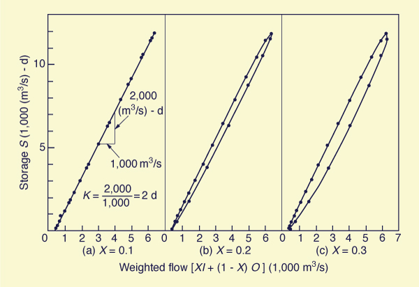
Several values of X are tried, within the range 0.0 to 0.5, for example, 0.1, 0.2 and 0.3.
For each trial value of X, the weighted flows [ XI + ( 1 - X ) O ] are calculated, as shown in Cols. 5-7.
Each of the weighted flows is plotted against channel storage (Col. 4), as shown in Fig. 10-16.
The value of X for which the storage versus weighted flow data plots closest to a line is taken as the correct value of X.
In this case, Fig. 10-16 (a): X = 0.1 is chosen.
Following Eq. 10-88, the value of K is obtained from Fig. 10-16 (a) by calculating the slope of the storage vs weighted outflow curve.
In this case, the value of K = [2000 (m3/s)-d]/(1000 m3/s) = 2 d.
Thus, it is shown that K = 2 days and X = 0.1 are the Muskingum routing parameters for the given inflow and outflow hydrographs.
Figure 10-16 Calibration of Muskingum routing parameters: Example 10-2. | |||||||||||||||||||||||||||||||||||||||||||||||||||||||||||||||||||||||||||||||||||||||||||||||||||||||||||||||||||||||||||||||||||||||||||||||||||||||||||||||||||||||||||||||||||||||||||||||||||||||||||||||||||
The estimation of routing parameters is crucial to the application of the Muskingum method. The parameters are not constant, tending to vary with flow rate. If the routing parameters can be related to flow and channel characteristics, the need for trial-and-error calibration would be eliminated. Parameter K could be related to reach length and flood wave velocity, whereas X could be related to the diffusivity characteristics of flow and channel. These propositions are the basis of the Muskingum-Cunge method.
10.6 MUSKINGUM-CUNGE METHOD
|
|
The Muskingum method requires a calibration in order to identify the routing parameters (Example 10-2). The procedure is based on measured input and output hydrographs, as shown in Cols. 2 and 3 of Table 10-5. Therefore, a gaging station is an absolute necessity for the Muskingum method to be properly used. This limits the applicability of the method to reaches which have a streamgaging station.
Unlike the Muskingum method, the Muskingum-Cunge method requires hydraulic rather than hydrologic data in order to calculate the routing parameters. The hydraulic data consists of geomorphic data such as channel slope and cross-sectional characteristics. Thus, the Muskingum-Cunge method does not explicitly require a streamgaging station, being applicable to any channel reach as long as the geomorphic data is available.
The Muskingum method is derived by combining the differential equation of storage, i.e., the continuity equation expressed in total differential form (Eq. 10-87) with a linear inflow-outflow-storage relation (Eq. 10-88). This leads to the Muskingum routing equation (Eq. 10-92) with appropriate routing coefficients (Eq. 10-93). The Muskingum-Cunge method is derived by discretizing the kinematic wave equation (Eq. 10-55) in a linear mode, in a manner similar to that of the Muskingum method, which leads to the same routing equation. The coefficients, however, are defined based on measurable channel characteristics.
The similarities appear to end there. The Muskingum method is lumped across the channel reach, based on storage, and able to describe flood wave diffusion (Example 10-1). The Muskingum-Cunge method is distributed, with data specified at cross sections, and based on a discretization of the kinematic wave equation, which ostensibly does not diffuse. Yet actual calculations using the Muskingum-Cunge method shows that it is able to describe wave diffusion, in a manner similar to the Muskingum method.
Cunge (1969) traced the diffusion of the discretized analog of the kinematic wave equation to the numerical diffusion of the scheme itself (see box). Thus, he was able to explain the paradox. The Muskingum and Muskingum-Cunge methods have the same theoretical basis. The routing parameters of the Muskingum method are hydrologic, based on storage, and determined by calibration using streamflow data. The routing parameters of the Muskingum-Cunge method are hydraulic, distributed (at a cross section), and based exclusively on geomorphic data.
|
A word of explanation on the concept of numerical diffusion 1
The existence of diffusion in a numerical scheme needs further elaboration. As Hayami (1951) pointed out, in nature irregularities produce physical diffusion. The same process extends to the computational world: Irregularities produce numerical diffusion. The irregularities are interpreted as the errors inherent to the numerical computation, among which the truncation errors stand out primordially. The replacement of a partial differential equation, based on ∂, with a finite difference equation, based on Δ, results in errors, which, when taken in the aggregate, manifest themselves as diffusion. Thus, numerical diffusion is in the computational world what physical diffusion is in the real world. 1 See Cunge (1969) for a detailed treatment of numerical diffusion in connection with the Muskingum method. |
Muskingum-Cunge routing equation
To derive the Muskingum-Cunge routing equation, the kinematic wave equation (Eq. 10-55) is discretized on the x-t plane (Fig. 10-17) in a way that parallels the Muskingum method, centering the spatial derivative and off-centering the temporal derivative by means of a weighting factor X:
|
X (Q j n+1 - Q j n ) + (1 - X) (Q j+1n+1 - Q j+1 n ) ________________________________________________ + Δt |
|
(Q j+1 n - Q j n ) + (Q j+1n+1 - Q
j n+1 ) c _______________________________________ = 0 2 Δx | (10-94) |
in which c = βV is the kinematic wave celerity.
Figure 10-17 Space-time discretization of the kinematic wave equation |

Solving Eq. 10-94 for the unknown discharge leads to the following routing equation:
| Q j+1 n+1 = C0 Q j n+1 + C1 Q j n + C2 Q j+1 n | (10-95) |
The routing coefficients are:
|
c ( Δt / Δx ) - 2X C0 = ________________________ 2(1 - X) + c ( Δt / Δx ) | (10-96a) |
|
c ( Δt / Δx ) + 2X C1 = ________________________ 2(1 - X) + c ( Δt / Δx ) | (10-96b) |
|
2(1 - X) - c ( Δt / Δx ) C2 = ________________________ 2(1 - X) + c ( Δt / Δx ) | (10-96c) |
By defining the travel time as
|
Δx K = ______ c | (10-97) |
it is seen that the sets of Eq. 10-93 and Eq. 10-96 are the same.
Equation 10-97 confirms that K is in fact the flood wave travel time, i.e., the time it takes a given discharge to travel the reach length Δx with the kinematic wave celerity c.
Numerical properties
The Courant number is defined as the ratio of physical celerity (c) to the numerical, or grid, celerity
|
Δt C = c ______ Δx | (10-98) |
Equation 10-95 is a numerical analog of Eq. 10-55 and, therefore, subject to numerical diffusion and dispersion. Numerical diffusion is the second-order error; numerical dispersion is the third-order error. The following conditions hold:
For X = 0.5 and C = 1, the routing equation is third-order accurate, i.e., the numerical solution is equal to the analytical solution (of the kinematic wave equation).
For X = 0.5 and C ≠ 1, the routing equation is second-order accurate, exhibiting only numerical dispersion.
For X < 0.5 and C ≠ 1, the routing equation is first-order accurate, exhibiting both numerical diffusion and dispersion.
For X < 0.5 and C = 1, the routing equation is first-order accurate, exhibiting only numerical diffusion.
These relations are summarized in Table 10-6.
| ||||||||||||||||||||||||||||||
In practice, the numerical diffusion can be used to simulate the physical diffusion of the actual flood wave. By expanding the discrete function Q (jΔx, n Δt) in Taylor series about grid point (jΔx, n Δt), the numerical diffusion coefficient of the Muskingum scheme is derived (Cunge, 1969) (Appendix B):
|
1 νn = c Δx ( ____ - X ) 2 | (10-99) |
in which νn is the numerical diffusion coefficient of the Muskingum scheme. This equation reveals the following:
For X = 0.5 there is no numerical diffusion, although there is some numerical dispersion for
C ≠ 1; For X > 0.5, the numerical diffusion coefficient is negative, i.e., numerical amplification, which explains the behavior of the Muskingum method for this range of X values;
For Δx = 0, the numerical diffusion coefficient is zero, clearly the trivial case.
A predictive equation for X can be obtained by matching the hydraulic diffusivity νh (Eq. 10-83) with the numerical diffusion coefficient of the Muskingum scheme νn (Eq. 10-99). This leads to the following expression for X:
|
1 qo X = ___ ( 1 - __________ ) 2 So c Δx | (10-100) |
With X calculated by Eq. 10-100, the Muskingum method is referred to as Muskingum-Cunge method. Thus, the routing parameter X can be calculated as a function of the following numerical and physical properties:
Reach length Δx,
Reference discharge per unit width qo,
Kinematic wave celerity c, and
Bottom slope So.
It should be noted that Eq. 10-100 was derived by matching physical and numerical diffusion (a second-order processes), and does not account for dispersion (a third-order process). Therefore, in order to simulate wave diffusion properly with the Muskingum-Cunge method, it is necessary to optimize numerical diffusion (with Eq. 10-100) while at the same time minimizing numerical dispersion by keeping the value of C ≅ 1.
|
Advantage of the Muskingum-Cunge method
A unique feature of the Muskingum-Cunge method, which sets it apart from other numerical kinematic wave models, is the grid independence of the calculated outflow hydrograph.
If numerical dispersion is minimized, the calculated outflow at the downstream end of a channel reach will be essentially the same, regardless of how many subreaches are used in the computation.
This is because X is a function of Δx,
and the routing coefficients C0, C1,
and |
An improved version of the Muskingum-Cunge method is due to Ponce and Yevjevich (1978). The grid diffusivity is defined as the numerical diffusivity for the case of X = 0. From Eq. 10-99, the grid diffusivity is:
|
Δx νg = c _____ 2 | (10-101) |
The cell Reynolds number D is defined as the ratio of hydraulic diffusivity (Eq. 10-83) to grid diffusivity (Eq. 10-101). This leads to:
|
qo D = __________ So c Δx | (10-102) |
Therefore:
|
1 X = ___ ( 1 - D ) 2 | (10-103) |
Equations 10-101 and 10-102 imply that for very small values of Δx, D may be greater than 1, leading to negative values of X. In fact, for the characteristic reach length
|
qo Δxc = ________ So c | (10-104) |
the cell Reynolds number is D = 1, and X = 0. Therefore, in the Muskingum-Cunge method, reach lengths shorter than the characteristic reach length result in negative values of X. This should be contrasted with the classical Muskingum method (Section 10.4), in which X is restricted in the range 0.0 ≤ X ≤ 0.5. In the classical Muskingum, X is interpreted as a weighting factor. As shown by Eqs. 10-101 and 10-102, nonnegative values of X are associated with long reaches, typical of the manual computation used in the development and early application of the Muskingum method.
In the Muskingum-Cunge method, however, X is interpreted in a moment-matching sense or diffusion-matching factor. Therefore, negative values of X are entirely possible. This feature allows the use of shorter reaches than would otherwise be possible if X were restricted to nonnegative values.
Routing coefficients
The substitution of Eqs. 10-98 and 10-100 into Eq. 10-96 leads to routing coefficients expressed in terms of Courant and cell Reynolds numbers:
|
-1 + C + D C0 = ______________ 1 + C + D | (10-105a) |
|
1 + C - D C1 = ______________ 1 + C + D | (10-105b) |
|
1 - C + D C2 = ______________ 1 + C + D | (10-105c) |
The calculation of routing parameters C and D can be performed in several ways. The wave celerity can be calculated with either Eq. 10-57 or Eq. 10-59. With Eq. 10-57, c = βV; with Eq. 10-59, c = (1/T) dQ/dy. Theoretically, these two equations are the same. For practical applications, if a stage-discharge rating and cross-sectional geometry are available (i.e., stage-discharge-top width tables), Eq. 10-59 is preferred over Eq. 10-57 because it accounts directly for cross-sectional shape. In the absence of a stage-discharge rating and cross-sectional data, Eq. 10-57 can be used to estimate flood wave celerity.
With the aid of Eqs. 10-98 and 10-102, the routing parameters may be based on flow characteristics. The calculations can proceed in a linear or nonlinear mode. In the linear mode, the routing parameters are based on reference flow values and kept constant throughout the computation in time. The choice of reference flow has a bearing on the calculated results, although the overall effect is likely to be small (Ponce and Yevjevich, 1978). For practical applications, either an average or peak flow value can be used as reference flow. The peak flow value has the advantage that it can be readily ascertained, although a better approximation may be obtained by using an average value. The linear mode of computation is referred to as the constant-parameter Muskingum-Cunge method to distinguish it from the variable-parameter Muskingum-Cunge method, in which the routing parameters are allowed to vary with the flow. The constant parameter method resembles the Muskingum method, with the difference that the routing parameters are based on measurable flow and channel characteristics instead of on historical streamflow data.
Example 10-3.
Use the constant-parameter Muskingum-Cunge method to route a flood wave with the following flood and channel characteristics: peak flow
Qp = 1000 m3/s; baseflow Qb, = 0 m3/s; channel bottom slope So =
0.000868; flow area at peak discharge Ap = 400 m2; top width at peak discharge Tp = 100 m;
rating exponent β = 1.6; reach length Δx = 14.4 km; time interval Δt = 1 h.
The mean velocity (based on the peak discharge) is V = Qp/Ap = 2.5 m/s.
The wave celerity is c = βV =
ONLINE CALCULATION.
Using ONLINE ROUTING05, the answer
is essentially the same as that of Col. 6, Table 10-7.
| |||||||||||||||||||||||||||||||||||||||||||||||||||||||||||||||||||||||||||||||||||||||||||||||||||||||||||||||||||||||||||||||||||||||
Resolution requirements
When using the Muskingum-Cunge method, care should be taken to ensure that the values of Δx and Δt are sufficiently small to approximate closely the actual shape of the hydrograph. For smoothly rising hydrographs, a minimum value of tp /Δt = 5 is recommended. This requirement usually results in the hydrograph time base being resolved into at least 15 to 25 discrete points, considered adequate for Muskingum routing.
Unlike temporal resolution, there is no definite criteria for spatial resolution. A criterion borne out by experience is based on the fact that Courant and cell Reynolds numbers are inversely related to reach length Δx. Therefore, to keep Δx sufficiently small, Courant and cell Reynolds numbers should be kept sufficiently large. This leads to the practical criterion (Ponce and Theurer, 1982):
| C + D ≥ 1 | (10-106) |
which can be written as follows: -1 + C + D ≥ 0. This confirms the necessity of avoiding negative values of C0 in Muskingum-Cunge routing (see Eq. 10-105a). Experience has shown that negative values of either C1 or C2 do not adversely affect the method's overall accuracy.
Notwithstanding Eq. 10-106, the Muskingum-Cunge method works best when the numerical dispersion is minimized, that is, when C ≅ 1. Values of C substantially less than 1 are likely to cause the notorious dips, or negative outflows, in portions of the calculated hydrograph. This computational anomaly is attributed to excessive numerical dispersion and should be avoided.
Nonlinear Muskingum-Cunge method
The kinematic wave equation, Eq. 10-55, is nonlinear because the kinematic wave celerity varies with discharge. The nonlinearity is mild, among other things because the wave celerity variation is usually restricted within a narrow range. However, in certain cases it may be necessary to account for this nonlinearity. This can be done in two ways: (1) during the discretization, by allowing the wave celerity to vary, resulting in a nonlinear numerical scheme to be solved by iterative means; and (2) after the discretization, by varying the routing parameters, as in the variable-parameter Muskingum-Cunge method (Ponce and Yevjevich, 1978). The latter approach is particularly useful if the overall nonlinear effect is small, which is often the case.
The variable parameter Muskingum-Cunge method represents a small yet sometimes perceptible improvement over the constant parameter method. The differences are likely to be more marked for very long reaches and/or wide variations in flow levels. Flood hydrographs calculated with variable parameters show a certain amount of distortion, either wave steepening in the case of flows contained inbank or wave attenuation (flattening) in the case of typical overbank flows. This is a physical manifestation of the nonlinear effect, i.e., different flow levels traveling with different celerities. On the other hand, flood hydrographs calculated using constant parameters do not show wave distortion.
Assessment of Muskingum-Cunge method
The Muskingum-Cunge method is a physically based alternative to the Muskingum method. Unlike the Muskingum method where the parameters are calibrated using streamflow data, in the Muskingum-Cunge method the parameters are calculated based on flow and channel characteristics. This makes possible channel routing without the need for time-consuming and cumbersome parameter calibration. More importantly, it makes possible extensive channel routing in ungaged streams with a reasonable expectation of accuracy. With the variable-parameter feature, nonlinear properties of flood waves (which could otherwise only be obtained by more elaborate numerical procedures) can be described within the context of the Muskingum formulation.
Like the Muskingum method, the Muskingum-Cunge method is limited to diffusion waves. Furthermore, the Muskingum-Cunge method is based on a single-valued rating and does not take into account strong flow non-uniformity or unsteady flows exhibiting substantial loops in discharge-stage rating (i.e., dynamic waves). Thus, the Muskingum-Cunge method is suited for channel routing in natural streams without significant backwater effects and for unsteady flows that classify under the diffusion wave criterion (Eq. 10-66).
An important difference between the Muskingum and Muskingum-Cunge methods should be noted. The Muskingum method is based on the storage concept (Eq. 10-87) and, therefore, it is lumped, with the parameters K and X being reach averages. The Muskingum-Cunge method, however, is distributed in nature, with the parameters C and D being based on values evaluated at channel cross sections. Therefore, for the Muskingum-Cunge method to improve on the Muskingum method, it is necessary that the routing parameters evaluated at channel cross sections be representative of the channel reach under consideration (Fig. 10-18).
Historically, the Muskingum method has been calibrated using streamflow data. On the contrary, the Muskingum-Cunge method relies on physical characteristics such as rating curves, cross-sectional data and channel slope. The different data requirements reflect the different theoretical bases of the methods, i.e., lumped storage concept in the Muskingum method, and distributed kinematic/diffusion wave theory in the Muskingum-Cunge method.
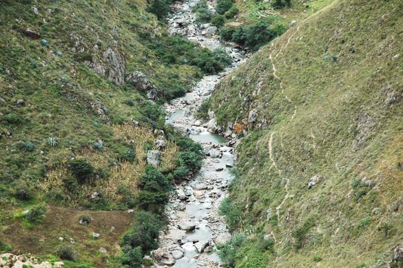
Figure 10-18 Moyan river, Lambayeque, Peru. |
10.7 DYNAMIC WAVES
|
|
In unsteady open-channel flow, the term dynamic wave is used to refer to two different types of waves:
A wave that neglects the friction and bottom slope, that is, wave [3] in Table 10-2, and
A wave that includes all terms in the equation of motion, that is, wave [5] in Table 10-2.
To avoid confusion, the first type of wave [3] is referred here as true dynamic wave. The second type [5] is referred to as mixed kinematic-dynamic wave, for short, mixed dynamic wave.
True dynamic waves
Conceptually, true dynamic waves are the exact opposite of kinematic waves. While kinematic waves lie to the left side of the wavenumber spectrum, true dynamic waves lie to the right (Fig. 10-3). Thus, their dimensionless wavenumber is long, that is, the wavelength L is short relative to the reference channel length Lo (Eq. 10-30).
While the dimensionless relative celerity of a kinematic wave is constant and equal to 0.5, that of the true dynamic wave is equal to the reciprocal of the Froude number (Fig. 10-3):
|
1 (gho)1/2 cdrd = ____ = _________ F uo | (10-107) |
The relative celerity of a true dynamic wave is:
|
crd = (gho)1/2 | (10-108) |
The celerity of a true dynamic wave is:
|
crd = uo ± (gho)1/2 | (10-109) |
Therefore, a true dynamic wave has two components, with celerities:
|
crd1 = uo + (gho)1/2 | (10-110) |
|
crd2 = uo - (gho)1/2 | (10-111) |
Kinematic and true dynamic waves share a distinct property: They do not attenuate. This is due to the constancy of the dimensionless relative wave celerity within the applicable range of dimensionless wavenumbers (Fig. 10-3).
In practice, true dynamic waves apply to the "short" waves that may be present in laboratory flumes and small canals. They do not apply for flood waves, which lie on the left side of the dimensionless wavenumber spectrum.
Mixed dynamic waves
Mixed kinematic-dynamic waves lie toward the middle of the wavenumber spectrum (Fig. 10-3). Conceptually, they are the most complete type of wave, because they consider all the terms in the equation of motion (Table 10-2). However, for Vedernikov numbers V < 1, (corresponding to Froude numbers F < 2 under Chezy friction in hydraulically wide channels), the mixed waves are subject to strong attenuation. The attenuation is strongest at the point of inflexion of the dimensionless relative celerity versus dimensionless wavenumber function (Fig. 10-3). Figure 10-4 shows the attenuation rates as described by the logarithmic decrement δ.
Lighthill and Whitham (1955) described the impermanence of dynamic waves in the following terms:
"In the case of flood waves, kinematic and dynamic waves are both possible together. However, the dynamic waves have both a much higher wave velocity and also a rapid attenuation. Hence, although any disturbance sends some signal downstream at the ordinary wave velocity for long gravity waves (sic), this signal is too weak to be noticed at any considerable distance downstream, and the main signal arrives in the form of a kinematic wave at a much slower velocity."
They followed up with this statement (op. cit., page 291):
"We have thought it desirable to give a mathematical treatment of the 'competition' between kinematic and dynamic waves in river flow, in order to show how completely the dynamic waves are subordinated in the case of greatest interest, that is, when the speed of the river is well subcritical. This demonstrates the unsuitability of the characteristics of the dynamic wave as the basis for computation."
Thus, in general, mixed dynamic waves do not apply to flood flows in natural streams. Once generated, dynamic waves tend to dissipate very quickly, with their mass going to join the predominant underlying kinematic or kinematic-with-diffusion (diffusion) wave.
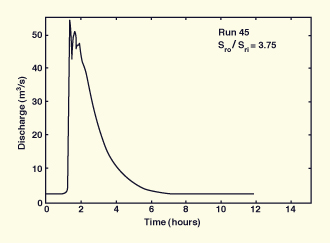
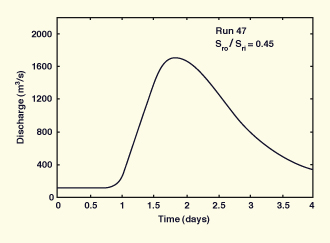
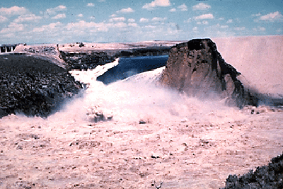
The exception may be a flood wave generated by a dam breach, which is typically so sudden that it may actually be a mixed dynamic wave. These waves attenuate very quickly, confirming the correctness of the theory. For example, consider the failure of Teton Dam, in Idaho, on June 5, 1976 (Fig. 10-19). The flood wave released at the damsite attenuated to a small fraction of its initial strength within a relatively short distance downstream. Many other examples of actual dam breaches have confirmed that dam-breach flood waves tend to dissipate rather quickly.
|
Modeling of mixed dynamic waves
In a dynamic wave solution, the equations of continuity and motion are solved by a numerical procedure, either (a) the method of finite differences, (b) the method of characteristics, or (c) the finite element method. In the method of finite differences, the partial differential equations are discretized following a chosen numerical scheme. The method of characteristics is based on the conversion of the set of partial differential equations into a related set of ordinary differential equations, and the solution along a characteristic grid, i.e. a grid that follows characteristic directions. The method of finite elements solves a set of integral equations over a chosen grid of finite elements.
In the past four decades, the method of finite differences has come to be regarded as the most expedient way of obtaining a (mixed) dynamic wave solution for practical applications. Among several numerical schemes that have been used in connection with the dynamic wave, the Preissmann scheme is perhaps the most popular (Liggett and Cunge, 1975). This is a four-point scheme, centered in the temporal derivatives and slightly off-centered in the spatial derivatives, by use of a weighting factor θ. The off-centering in the spatial derivatives introduces a small amount of numerical diffusion necessary to control the numerical stability of the nonlinear scheme. This produces a workable yet sufficiently accurate scheme.
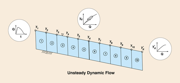
The independent variables used in (mixed) dynamic wave routing are usually discharge Q and
Figure 10-20 Reach subdivision for dynamic wave routing. |
In practice, a (mixed) dynamic wave solution represents an order-of-magnitude increase in complexity and associated data requirements when compared to either kinematic or diffusion wave solutions. Its use is recommended in situations where neither kinematic nor diffusion wave solutions are likely to adequately represent the physical phenomena. In particular, (mixed) dynamic wave solutions are applicable to dam-breach flood waves, flow over very flat slopes, flow into large reservoirs, strong backwater conditions and flow reversals. In general, the (mixed) dynamic wave is recommended for cases warranting a precise determination of the unsteady variation of river stages.
The current version (Version 4.1) of the U.S. Army Corps of Engineers' HEC-RAS model (U.S. Army Corps of Engineers, 2010) contains a dynamic wave module suited for practical applications.
Mixed dynamic rating curve
Mixed dynamic wave solutions are often referred to as hydraulic river routing. As such, they have the capability to calculate unsteady discharges and stages when presented with the appropriate geometric channel data and initial and boundary conditions. Their importance in unsteady flow is examined here by comparing them to kinematic and diffusion waves.
Kinematic waves calculate unsteady discharges; the corresponding stages are subsequently obtained from the appropriate rating curves. Equilibrium (steady, uniform) rating curves are used for this purpose. Diffusion waves may or may not use equilibrium rating curves to calculate stages. Some methods, e.g., Muskingum-Cunge, use equilibrium ratings, but more elaborate diffusion wave solutions may not.
Mixed dynamic waves rely on the physics of the phenomena as built into the governing equations to generate their own unsteady flow rating. A looped rating curve is produced at every cross section, as shown in Fig. 10-21. For any given stage, the discharge is higher in the rising limb of the hydrograph and lower in the receding limb. This loop is due to hydrodynamic reasons and should not be confused with other loops, which may be due to erosion, sedimentation, or changes in bed configuration.
Figure 10-21 Sketch of the looped rating of dynamic waves. |
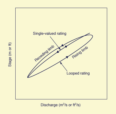
The width of the loop is a measure of the flow unsteadiness, with wider loops corresponding to highly unsteady flow. If the loop is narrow, it implies that the flow is mildly unsteady, perhaps a diffusion wave. If the loop is practically nonexistent, the flow can be approximated as kinematic flow. In fact, the basic assumption of kinematic flow is that momentum can be simulated as steady uniform flow, i.e., that the rating curve is single-valued.
The preceding observations lead to the conclusion that the importance of mixed dynamic waves is directly related to the flow unsteadiness and the associated loop in the rating curve. For highly unsteady flows such as dam-breach flood waves, it may well be the only way to properly account for the looped rating. For other less unsteady flows, kinematic and diffusion waves are a viable alternative, provided their applicability can be clearly demonstrated.
Downstream boundary condition
Modeling of a mixed dynamic wave presents an interesting paradox: In order to solve the problem correctly, a dynamic downstream boundary condition (usually a rating curve) must be specified. However, a dynamic downstream boundary condition is not known a priori. Abbott (1976) put it in the right perspective when he stated:
"A common source of error is the use of a boundary condition in a dynamic model that is really only proper to a pure kinematic model... but in a dynamic model the solution itself generates different discharge-stage relations according to the variabilities of the flows, so that a unique relation at the boundary contradicts the solution within the boundary. A finely balanced model will usually go unstable in this situation, but models with heavy numerical damping may survive, only to give erroneous results."
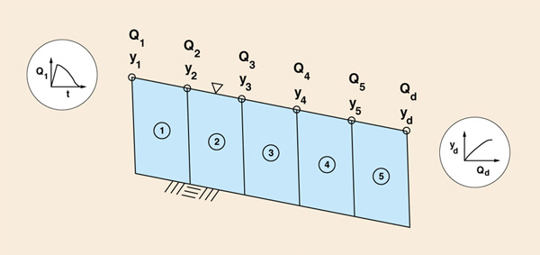
A way out of this difficulty is to artificially extend the channel several subreaches downstream, and to specify a kinematic rating at the newly defined downstream boundary, while giving the loop a chance to develop at the upstream cross section of interest (Fig. 10-22). Ponce and Lugo (2001) have used sensitivity analysis to show that the artificial extension of the channel by an amount equal to the channel length (i.e., doubling the channel length) may be sufficient to produce an accurate looped rating at the cross section of interest.
Figure 10-22 Artificial extension of the computational domain, for use in mixed dynamic wave |
QUESTIONS
|
|
What conservation laws are used in the description of steady gradually varied flow?
What conservation laws are used in the description of unsteady gradually varied flow?
What forces are acting in a control volume in unsteady gradually varied flow?
What waves types are common in unsteady open-channel flow?
To what problems do kinematic waves apply?
To what problems do diffusion waves apply?
How is Lo defined?
What is the dimensionless wavenumber?
What is the dimensionless relative celerity of kinematic waves under Chezy friction in hydraulically wide channels?
What is the dimensionless relative celerity of dynamic waves under Chezy friction in hydraulically wide channels?
What are three ways of expressing the convective celerity of kinematic waves?
What is the neutral-stability Froude number for triangular channels with Chezy friction?
What is the neutral-stability Froude number for hydraulically wide channels with Manning friction?
What is the basis of the Muskingum-Cunge method?
What is Hayami's contribution to flood routing?
For what value of Vedernikov number are kinematic and dynamic hydraulic diffusivities the same?
For what value of Vedernikov number does the dynamic hydraulic diffusivity vanish?
What part of the flood routing does the Muskingum parameter X account for?
What is numerical diffusion?
What is numerical dispersion?
What is the advantage of the Muskingum-Cunge method?
When will the Muskigum-Cunge method fail to give good results?
How is the downstream boundary specified in a mixed kinematic-dynamic model if increased accuracy is desired?
PROBLEMS
|
|
You are observing the rise of a river during flood. The width of the river at the observation point, and for some distance upstream is 65 m, and according to the gage reading, the discharge is Q = 70 m3/s. Estimate the discharge at a point located 15.875 km upstream, if the water surface is rising at the rate of 9 mm/hr at your location and at 12 mm/hr at the upstream cross section.
A hydraulically wide channel is operating at Froude number F = 0.22. The unit-width discharge is q = 2.8 m2/s. What are the two absolute Lagrange celerities?
A flood wave is traveling inbank through a straight river reach of top width T = 320 m wide and length L = 5625 m. For every 1 cm of flood rise, the discharge goes up 10 m3/s. How long will it take for a given discharge to travel the length of the reach?
Calculate the exponent β of the discharge-area rating for a triangular channel with Chezy friction.
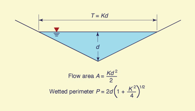
Fig. 10-23 Definition sketch for a triangular channel.
Calculate the exponent β of the discharge-area rating for a triangular channel with Manning friction.
A flood hydrograph has the following data: time-of-rise tr = 2 hr, reference velocity Vo = 2 ft/s, reference flow depth do = 6 ft, bottom slope So = 0.004. Determine is this wave is a kinematic wave.
A flood hydrograph has the following data: time-of-rise tr = 2 hr, reference velocity Vo = 2 ft/s, reference flow depth do = 6 ft, bottom slope So = 0.004. Determine is this wave is a diffusion wave.
A flood hydrograph has the following data: time-of-rise tr = 1 hr, reference velocity Vo = 2 m/s, reference flow depth do = 2 m, bottom slope So = 0.0004. Determine is this wave is a diffusion wave.
Using ONLINE ROUTING 04, route a flood wave using the Muskingum method. The inflow hydrograph ordinates are [25 ordinates, starting at time = 0, to time = 24 hr]:
100, 130, 150, 180, 220, 250, 300, 360, 450, 550, 700, 550, 490, 370, 330, 310, 280, 230, 170, 150, 130, 120, 110, 105, 100.
Assume Δt = 1 hr, K = 1 hr, X = 0.3. Report the peak outflow and time of occurrence.
Using ONLINE ROUTING 05, route the same flood wave as the previous problem using the Muskingum-Cunge method. Use the following input data: Qp = 700 m3/s, Ap = 400 m2,
Tp = 88 m, Δt = 1 hr, Δx = 9.6 km, β = 1.65, So = 0.0007. Report the peak outflow and time of occurrence.
REFERENCES
|
|
Abbott, M. A. 1976. Computational hydraulics: A short pathology. Journal of Hydraulic Research, Vol. 14, No. 4, p. 276.
Chow, V. T. 1959. Open-channel Hydraulics. McGraw Hill, New York.
Craya, A. 1952. The criterion for the possibility of roll-wave formation. Gravity Waves, Circular No. 521, National Bureau of Standards, Washington, D.C. 141-151.
Cunge, J. A. (1969). On the Subject of a Flood Propagation Computation Method (Muskingum Method), Journal of Hydraulic Research, Vol. 7, No. 2, 205-230.
Dooge, J . C. I. 1973. Linear theory of hydrologic systems. Technical Bulletin No. 1468, U.S. Department of Agriculture, Washington, D.C.
Hayami, I. 1951. On the propagation of flood waves. Bulletin, Disaster Prevention Research Institute, No. 1, December.
Kibler, D. F., and D. A. Woolhiser. 1970. The kinematic cascade as a hydrologic model. Hydrology Paper No. 39, Colorado State University, Ft. Collins, Colorado.
Kleitz, M. 1877. Note sur la théorie du mouvement non permanent des liquides et sur application à la propagation des crues des rivières, (Note on the theory of unsteady flow of liquids and on application to flood propagation in rivers), Annals des Ponts et Chaussées, ser. 5, Vol. 16, 2e semestre, 133-196.
Liggett, J. A. 1975. Basic equations of unsteady flow. Chapter 2 in Unsteady flow in open channels, K. Mahmood and V. Yevjevich, eds., Water Resources Publications, Ft. Collins, Colorado.
Liggett, J. A., and J. A. Cunge. 1975. Numerical methods of solution of the unsteady flow equations. Chapter 4 In Unsteady flow in open channels, K. Mahmood and V. Yevjevich, eds., Water Resources Publications, Ft. Collins, Colorado.
Lighthill, M. J., and G. B. Whitham. 1955. On kinematic waves: I. Flood movement in long rivers. Proceedings, Royal Society of London, Series A, 229, 281-316.
McCarthy, G. T. (1938). "The Unit Hydrograph and Flood Routing," unpublished manuscript, presented at a Conference of the North Atlantic Division, U.S. Army Corps of Engineers, June 24.
Ponce, V, M., and D. B. Simons. 1977. Shallow wave propagation in open-channel flow. Journal of the Hydraulics Division, ASCE, Vol. 103, No. HY12, December, 1461-1476.
Ponce, V. M., and V. Yevjevich. 1978. Muskingum-Cunge method with variable parameters. Journal of the Hydraulics Division, ASCE, Vol. 104, No. HY12, December, 1663-1667.
Ponce, V. M., and F. D. Theurer. 1982. Accuracy criteria in diffusion routing. Journal of the Hydraulics Division, ASCE, Vol. 108, No. HY6, June, 747-757.
Ponce, V, M., and D. Windingland. 1985. Kinematic shock: Sensitivity analysis. Journal of Hydraulic Engineering, ASCE, Vol. 111, No. 4, April, 600-611.
Ponce, V. M. 1989. Engineering hydrology: Principles and practices. Prentice Hall, Englewood Cliffs, New Jersey.
Ponce, V. M. 1990. Generalized diffusion wave equation with inertial effects. Water Resources Research, Vol. 26, No. 5, May, 1099-1101.
Ponce, V. M. 1991. New perspective on the Vedernikov number. Water Resources Research, Vol. 27, No. 7, 1777-1779, July.
Ponce, V, M., and P. J. Porras. 1995. Effect of cross-sectional shape of free-surface instability. Journal of Hydraulic Engineering, ASCE, Vol. 121, No. 4, April, 376-380.
Ponce, V, M., and A. Lugo. 2001. Modeling looped ratings in Muskingum-Cunge routing. Journal of Hydrologic Engineering, ASCE, Vol. 6, No. 2, March-April, 119-124.
Saint-Venant, B. de. 1871. Theorie du mouvement non-permanent des eaux avec application aux crues des rivieres et l' introduction des varees dans leur lit, Competes Rendus Hebdomadaires des Seances de l'Academie des Science, Paris, France, Vol. 73, 1871, 148-154.
Seddon, J. A. 1900. River hydraulics. Transactions, ASCE, Vol. XLIII, 179-243, June.
U.S. Army Corps of Engineers. 2010. River Analysis System: HEC-RAS, Version 4.1, Hydrologic Engineering Center, Davis, California.
| http://openchannelhydraulics.sdsu.edu |
|
140901 20:45 |