4.1  CRITICAL FLOW

[Computation of Critical Flow]   [Critical Flow Control]   [Sharp-crested Weirs]   [Questions]   [Problems]   [References]   •   [Top]

In open-channel flow, two characteristic thresholds describe the state of flow (Section 1.3):

1. Critical flow, which describes steady flow at Froude number F = 1, and

2. Neutrally stable flow, which describes the onset of flow instability, which occurs at Vedernikov number V = 1.

The ratio V/F embodies two important properties:

1. The type of friction, and

2. The type of cross-sectional geometry, or shape.

The discharge-flow area rating, Eq. 1-4, is repeated here for convenience:

Q = α Aβ

(4-1)

in which α = coefficient of the rating, and β = exponent. The latter is defined as follows (Section 1.3):

V β  = 1  +   _____                    F

(4-2)

Values of Froude number F corresponding to values of Vedernikov number V = 1, i.e., values of F_ns, are listed in Table 1-1.

Critical flow criterion

Critical flow occurs under the following conditions (Fig. 4-1):

• For a given discharge Q, when the specific energy E is a minimum.

• For a given specific energy E, when discharge Q is a maximum.

• For a given discharge Q, when the specific force F is a minimum.

• For a given specific force F, when discharge Q is a maximum.

• When the mean flow velocity u is equal to the relative celerity w of small surface perturbations, i.e., dynamic waves (Section 1.3).

• When the velocity head h_v is equal to one-half of the hydraulic depth D.

• When the Froude number F  is equal to 1.

Fig. 4-1  Critical flow over emergency spillway, Turner reservoir, San Diego County, California.

The condition of critical flow represents a threshold between subcritical flow, for which F < 1, and supercritical flow, for which F > 1.

Dynamic waves in open-channel flow have two components: (1) primary, and (2) secondary (Ponce and Simons, 1977). Primary waves travel with absolute velocity:

v1 = u  +  w

(4-3)

Secondary wave travels with absolute velocity:

v2 = u  -  w

(4-4)

While primary waves always travel downstream, secondary waves may travel upstream or downstream, depending on the flow conditions. In subcritical flow, w > u, and secondary waves are able to travel upstream. In supercritical flow, w < u, and secondary waves cannot travel upstream, instead traveling downstream. In practice, this means that subcritical flow is controlled from downstream, because surface perturbations are able to travel upstream. Conversely, supercritical flow cannot be controlled from downstream, because surface perturbations are not able to travel upstream. Instead, supercritical flow can be controlled only from upstream.

Critical flow may occur in one of two distinct modes:

1. Along the channel, under uniform flow, in what is referred to as critical uniform flow. The slope of the channel that sustains critical uniform flow is referred to as the critical slope.

2. At a specific cross section, under gradually varied flow upstream and downstream, in what is referred to as the critical cross section. [Actually, in the proximity of the critical flow cross section, the flow may be rapidly varied (Section 3.3)]. At a critical cross section, the flow depth is referred to as the critical depth (Fig. 4-2).

Fig. 4-2  Critical flow over a natural weir formed after stream degradation to bedrock, Aguaje de la Tuna, Tijuana, Baja California, Mexico.

The Darcy-Weisbach equation for open channel flow

The Darcy-Weisbach equation for open channel flow, Eq. 1-32, is repeated here for convenience (Section 1.4):

f        D S  =  ___   _____   F 2           8       R

(4-5)

in which the Froude number is:

V F  =  __________            (gD)1/2

(4-6)

For a hydraulically wide channel, for which D ≅ R, Eq. 4-5 reduces to:

f        S  =  ___   F 2           8

(4-7)

For application to open-channel flow, a modified Darcy-Weisbach friction factor f, equal to 1/8 of the usual Darcy-Weisbach friction factor f is applicable. The modified Darcy-Weisbach equation for open-channel flow is:

S  =  f F 2

(4-8)

Physical meaning of the critical slope

The critical slope is that for which F = 1. In Eq. 4-5, for F = 1:

f        D Sc  =  ___   _____             8       R

(4-9)

in which S_c = critical slope. In Eq. 4-7, for F = 1:

f         Sc  =  ___               8

(4-10)

Furthermore, in Eq. 4-8, for F = 1:

Sc  =  f

(4-11)

Equations 4-9 to 4-11 confirm that the friction factor and the critical slope are indeed closely related. For a channel of arbitrary cross section, Eq. 4-9 is applicable; for a hydraulically wide channel, Eq. 4-10 is applicable. When the modified Darcy-Weisbach friction factor f is used, Eq. 4-11 is applicable.

In general:

S  =  Sc F 2

(4-12)

in which S_c  is appropriately defined by either Eqs. 4-9, 4-10, or 4-11.

Equation 4-12 constitutes a type of Darcy-Weisbach equation applicable to open-channel flow. In uniform flow, this equation provides an enhanced physical meaning to the concept of critical slope. In gradually varied flow, Eq. 4-12 enables an increased understanding of the asymptotic limits to the water surface profiles (Section 7.3).

The following conclusions are drawn from Eq. 4-12:

Relationship between bottom slope, critical slope and Froude number The bottom slope is directly proportional to the Froude number, when the constant of proportionality is the critical slope. The bottom slope is directly proportional to the critical slope, when the constant of proportionality is the Froude number. The critical slope is inversely proportional to the Froude number, when the constant of proportionality is the bottom slope.

Occurrence of critical flow

As Eq. 4-12 indicates, critical flow occurs when the discharge is such that the critical slope (friction slope) equals the bottom slope. This is possible in a lined channel of fixed geometry, where as discharge increases, the friction slope eventually decreases to match the bottom slope. Thus, in an artificial prismatic channel, it is possible to achieve critical, and even supercritical, flow depths. Supercritical flows are rare, but not unheard of. For example, under Chezy friction in hydraulically wide channels, roll waves form under Vedernikov number V = 1, which corresponds to Froude number F = 2 (Fig. 1-6 and Table 1-1).

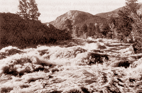
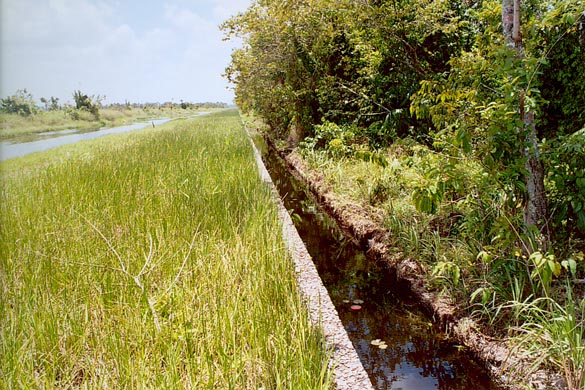
The situation is quite different in a natural channel, where the flow is able to freely interact with the boundary, increasing the "actual" or effective friction slope. In practice, the friction slope is not able to decrease to match the bottom slope, with the actual flow remaining subcritical, at least through most of its domain. Thus, as argued by Jarrett (1982), it is extremely rare to have critical or supercritical flow in a natural channel (Fig. 4-3).

ASCE Fig. 4-3  Arkansas River near Buena Vista, Colorado, with F < 1.

4.2  COMPUTATION OF CRITICAL FLOW

[Critical Flow Control]   [Sharp-crested Weirs]   [Questions]   [Problems]   [References]   •   [Top]   [Critical Flow]

From Eq. 4-6, the square of the Froude number is:

V 2 F 2  =  _______               gD

(4-13)

In Eq. 4-13, replacing V = Q /A and D = A /T  leads to:

Q 2 T F 2  =  _______              g A 3

(4-14)

At critical flow, F = 1, and Eq. 4-14 is conveniently expressed in the following form:

Q 2 Tc ________  -  Ac 3  =  0      g

(4-15)

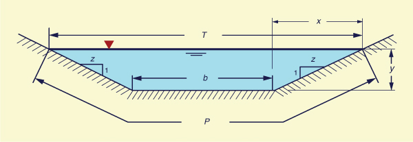
With reference to Fig 4-4, the top width T is:

T = b  +  2zy

(4-16)

The flow area A is:

A  =  (b  + x ) y  =  (b  + zy ) y

(4-17)

Fig. 4-4  Definition sketch for a trapezoidal cross section.

Replacing Eqs. 4-16 and 4-17 into Eq. 4-15:

Q 2 (b  +  2zyc) ________________  -  [ (b  + zyc ) yc ] 3  =  0              g

(4-18)

Given g = gravitational acceleration, and input data consisting of discharge Q, bottom width b, and side slope z [z:H to 1:V, Fig. 4-3], Eq. 4-18 is solved for the critical depth y_c . Then:

Tc = b  +  2zyc

(4-19)

Ac = (b  + zyc ) yc

(4-20)

Ac Dc  =  ______              Tc

(4-21)

Q Vc  =  ______              Ac

(4-22)

Equation 4-18 is expressed as follows:

Q 2 (b  +  2zyc) f (yc)  =  _________________  -  [ (b  + zyc ) yc ] 3                           g

(4-23)

Equation 4-23 is the general formula for critical flow, applicable to trapezoidal channels. For a rectangular channel: z = 0. Likewise, for a triangular channel of symmetrical section: b = 0.

In Eq. 4-23, making the change of variable x = y_c  for simplicity:

Q 2 (b  +  2zx) f (x)  =  ________________  -  [ (b  + zx ) x ] 3                          g

(4-24)

The solution of the cubic Eq. 4-24 may be accomplished by a trial-and-error procedure. A time-tested algorithm for the approximation to the first root of the equation is described below.

Critical flow algorithm Assume an initial value of x = 0. Then f(0) = Q2b/g, a large positive number. It is confirmed that the initial value of the function is greater than zero. Assume an initial value of the trial interval Δx = 1. Set x = x + Δx Calculate f (x) Stop when Δx < Δx TOL. A typical value of Δx TOL is 0.0001. If f (x) > 0, return to Step 3. if f (x) < 0, set Δx = 0.1 Δx Set x = x - 9 Δx Return to Step 4.

Critical depth in a hydraulically wide channel

For a hydraulically wide channel, or else, a rectangular channel: Q = qb, and z = 1. Replacing these values is Eq. 4-18 leads to an expression for critical depth y_c in terms only of unit-width discharge q :

q2 yc  =   ( ____ ) 1/3                g

(4-25)

Example 4-1. Using ONLINE CHANNEL 02, calculate the critical flow depth for the following flow conditions: Q = 10 m3/s; b = 5 m; z = 1.   ONLINE CALCULATION. Using the ONLINE CHANNEL 02 calculator, the critical depth is yc = 0.706 m; the critical velocity is vc = 2.482 m/s.

Example 4-2. Using ONLINE CHANNEL 02, calculate the critical flow depth for the following flow conditions: Q = 100 ft3/s; b = 12 ft; z = 0.   ONLINE CALCULATION. Using the ONLINE CHANNEL 02 calculator, the critical depth is yc = 1.292 ft; the critical velocity is vc = 6.448 ft/s.

4.3  CRITICAL FLOW CONTROL

[Sharp-crested Weirs]   [Questions]   [Problems]   [References]   •   [Top]   [Critical Flow]   [Computation of Critical Flow]

In Eq. 4-23, the critical flow depth is a function only of Q, b, and z. Thus, the critical flow depth, and for that matter, critical flow, is independent of the bottom slope and channel friction. Note that in Eq. 4-12, for F = 1, the critical slope effectively cancels with the bottom slope. Thus, in critical flow, the flow depth is independent of the slope and is, therefore, a constant for a given discharge.

The unique discharge-flow area (and unique discharge-stage rating), i.e., only one flow depth for every discharge, and vice versa, is referred to as control. Control can be either of types: (1) section control (transversal control), acting at a cross section, or (2) channel control (longitudinal control), acting along the channel.

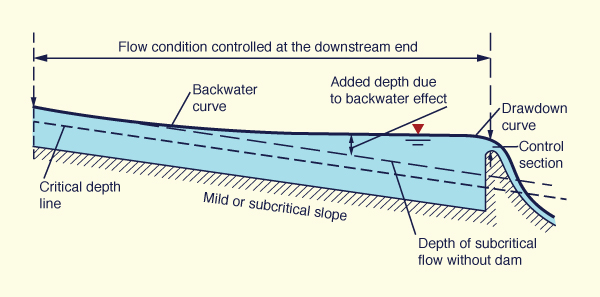
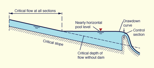
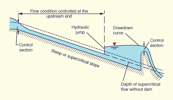
Figures 4-5 to 4-7 shows three cases of critical flow control in a prismatic channel, under the following slopes: (1) subcritical, (2) critical, and (3) supercritical.

The subcritical flow condition depicted on Fig. 4-5 shows the existence of critical section control only at the downstream dam crest. Thus, the flow is controlled at the downstream end.

Fig. 4-5  Location of critical control section in subcritical flow (Chow, 1959).

The critical flow condition of Fig. 4-6 shows critical control in two places: (1) section control at the downstream dam crest, and (2) channel control along the upstream critical slope channel. As shown, a backwater profile, which is a nearly horizontal pool level, connects the two flow control sections. The flow is controlled at the downstream end.

Fig. 4-6  Location of critical control section in critical flow (Chow, 1959).

The supercritical flow condition of Fig. 4-7 shows critical control in two places: (1) section control at the downstream dam crest, and (2) section control at the very upstream section of the supercritical channel. The flow is controlled at both downstream and upstream ends, with a hydraulic jump occurring somewhere in the middle.

Fig. 4-7  Location of critical control sections in supercritical flow (Chow, 1959).

The concept of uniqueness of the rating qualifies critical flow as a (section or channel) control. This provides an expedient way of determining discharge from stage, or stage from discharge, if one or the other is known. This property of critical flow is useful in flow measurements.

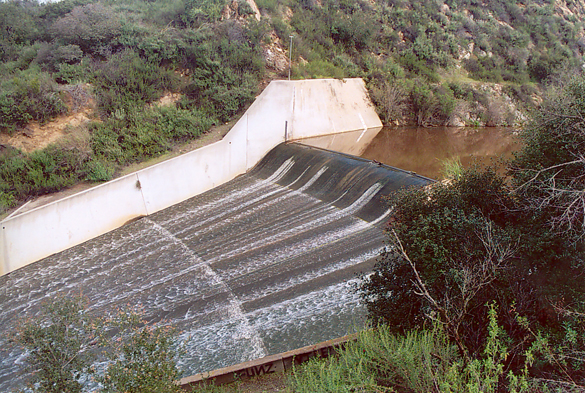
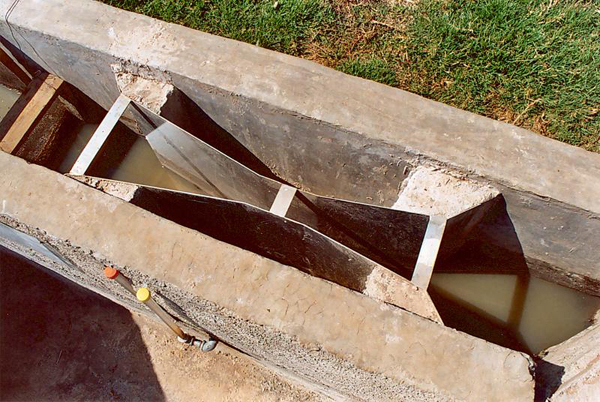
In practice, critical control for flow measurement is accomplished in two ways: (1) weir flow (section control), and (2) critical flow flume (channel control). Weir flow is described in Section 4-4. A typical example of a critical flow flume is the Parshall flume (Fig. 4-8). Under free-flowing conditions (low tailwater depth), only one gage measurement is required to determine the discharge. However, under submerged conditions (with high tailwater depth), two gage measurements are required.

Fig. 4-8  Parshall flume, Cucuchucho constructed wetland, Michoacan, Mexico.

In a broad-crested weir, critical flow occurs in the vicinity of the crest. The discharge per unit of width is:

q  =  Vc yc

(4-26)

q  =  (gyc)1/2 yc

(4-27)

q  =  (g)1/2 (yc)3/2

(4-28)

By definition, the critical depth is 2/3 of the total head H measured above the weir crest:

yc  =  (2/3) H

(4-29)

Replacing Eq. 4-29 in Eq. 4-28:

q  =  C H 3/2

(4-30)

in which C is a discharge coefficient defined as follows:

C  =  (2/3)3/2 g1/2

(4-31)

In SI units, C = 1.704; in U.S. Customary units, C = 3.087.

For various reasons, an actual design value C_d may differ from the theoretical value C. Experience has shown that the approximate range is: 0.8 ≤ C_d /C ≤ 1.3. Figure 4-9 shows a broad-crested weir for which C_d = 1.45 (SI units).

In practice, H is taken as the elevation of the water surface above the weir crest. This assumes that the approach velocity V_a at a section sufficiently upstream from the weir is zero: V_a = 0.

[See also Lab video:  The broad-crested weir].

Fig. 4-9  The 8,000-ft long overflow spillway weir at the Boerasirie Conservancy, Guyana.

4.4  SHARP-CRESTED WEIRS

[Questions]   [Problems]   [References]   •   [Top]   [Critical Flow]   [Computation of Critical Flow]   [Critical Flow Control]   [Sharp-crested Weirs]

Sharp-crested weirs are used to force section control in an open channel, for purposes of flow measurement. In practice, sharp-crested weirs have been built using: (1) triangular, (2) trapezoidal, or (3) rectangular sections.

Triangular weirs

Triangular weirs can be of two types: (a) fully contracted, or (b) partially contracted. Contraction refers to the size of the weir flow area as compared to the size of the approach channel flow area. Depending on size and design, a weir may be subject to both vertical and horizontal contraction. For a weir to be fully contracted, the ends of the weir should be sufficiently far from the sides and bottom of the approach channel (Fig. 4-10). Full contraction increases the measurement accuracy by providing a more precise channel control (a unique discharge-stage relation) in the immediate vinicity of the weir.

Fully contracted V-notch weir. The V-notch weir is a commonly used type of triangular sharp-crested weir. For V-notch weirs, full contraction is produced when the distance b from each side of the weir notch to each side of the weir pool is greater than 2H. For a 90° V-notch weir, the flow width at head level is equal to 2H. Therefore, the weir may be considered to be fully contracted when the ratio B/H > 6, i.e., for H/B < 0.167. For a 60° notch weir, the requirement for a fully contracted weir is: H/B < 0.194. In USBR practice, this translates into the practical criterion for a fully contracted V-notch weir: H/B ≤ 0.2.

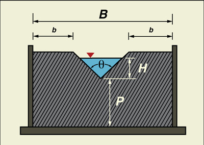
A weir not satisfying the above criterion is partially contracted, i.e., the approach channel width B is too narrow relative to the head H. In USBR practice, the practical criterion for a partially contracted V-notch weir is: H/B ≤ 0.4.

Fig. 4-10  V-notch weir schematic.

The fully contracted V-notch weir formula, in U.S. Customary units (Q in cfs, H in ft), is (USBR Water Manual):

Q = 4.28 Ce tan (θ/2) (H + k)5/2

(4-32)

In Eq. 4-32, the discharge Q is a function of hydraulic head H and angle θ. The discharge coefficient C_e and head correction coefficient k are a funtion of θ. The width of the approach channel B is used to check to see if the weir is fully contracted:  H/B ≤ 0.2.

The formula (polinomial fit) for C_e, with θ in degrees, is:

Ce = 0.607165052 - 0.000874466963 θ + 0.0000061039334 θ2

(4-33)

The formula (polinomial fit) for k, with θ in degrees, is (LMNO Engineering):

k = 0.0144902648 - 0.00033955535 θ + 0.00000329819003 θ2 - 0.0000000106215442 θ3

(4-34)

The fully contracted V-notch weir is restricted to the following conditions:

1. Head H < 1.25 ft (38 cm).

2. Width B > 3 ft (91 cm).

3. Height P > 1.5 ft (46 cm).

4. Ratio b/H ≥ 2.0.

5. Head/width ratio H/B ≤ 0.2.

Partially contracted V-notch weir. For the partially contracted 90° V-notch weir, Eq. 4-32 reduces to:

Q = 4.28 Ce (H + 0.0029)5/2

(4-35)

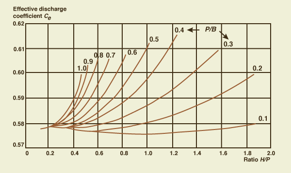
The discharge coefficient C_e is a function of the ratios H/P and P/B, as shown in Fig. 4-11.

Fig. 4-11  Variation of Ce as a function of H/P and P/B.

The formula for the partially contracted 90° V-notch weir is subject to the following restrictions:

1. Head H < 2 ft (61 cm).

2. Width B > 2 ft (61 cm).

3. Height P > 0.33 ft (10 cm).

4. Head/width ratio H/B ≤ 0.4.

Example 4-3. Using ONLINE VEE NOTCH 1, calculate the discharge over a fully contracted V-notch weir for the following flow conditions: Head H = 1 ft; width B = 6 ft; width b = 2 ft; angle θ = 90°.   ONLINE CALCULATION. Using the ONLINE VEE NOTCH 1 calculator, the discharge is: Q = 2.49 ft3/s.

Trapezoidal weir:  Cipolletti weir

A standard Cipolletti weir is trapezoidal in shape (Fig. 4-12). The crest and sides of the weir plate are placed far enough from the bottom and sides of the approach channel to produce full contraction. The sides incline outwardly at a slope of 1 horizontal to 4 vertical. The computation procedure follows Section 12 of Chapter 7 of the USBR Water Measurement Manual.

Fig. 4-12  Cipolletti weir schematic.

The formula for the Cipolletti weir, in U.S. Customary units, is:

Q = 3.367 L H 3/2

(4-36)

in which L = length of the weir crest, in ft, and H = head on the weir crest, in ft.

The accuracy of measurements obtained by Eq. 4-36 is considerably less than that obtainable with V-notch weirs. The accuracy of the discharge coefficient is ± 5 percent.

The Cipolletti weir is subject to the following restrictions:

1. The head H ≥ 0.2 ft (6.1 cm).

2. The ratio P/H ≥ 2.

3. The ratio b/H ≥ 2.

The head H is measured at a distance of at least 4H upstream from the crest.

Rectangular weirs

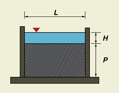
A rectangular weir has a rectangular shape, as shown in Fig. 4-13. To produce full contraction, the crest and sides of the weir plate are placed sufficiently far enough from the bottom and sides of the approach channel. The computation procedure follows Section 6 of Chapter 7 of the USBR Water Measurement Manual.

Fig. 4-13  Three-dimensional perspective of a rectangular weir.

The Kindsvater-Carter formula for a rectangular weir, in U.S. Customary units, is:

Q = Ce (L + kb) (H + 0.003)3/2

(4-37)

in which C_e = effective coefficient of discharge; L = length of the weir crest, in ft, k_b = a correction factor to obtain effective weir length, in ft; H = head measured above the weir crest, in ft; and Q = discharge, in cfs. The value B is the average width of the approach channel.

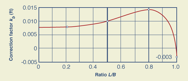
The correction factor k_b is a function of the ratio L/B, as shown in Fig. 4-14.

Fig. 4-14  Correction factor kb to obtain effective weir length.

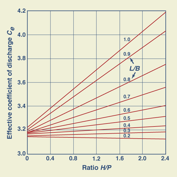
The effective coefficient of discharge C_e includes effects of relative depth and relative width of the approach channel. It is a function of H/P and L/B, as shown in Fig. 4-15.

Fig. 4-15  Values of Ce as a function of H/P and L/B.

Given H, L, B and P, and the ratios H/P and L/B, the computation proceeds with the following steps:

1. The correction factor k_b is calculated using Fig. 4-14.

2. The effective coefficient of discharge C_e is calculated using Fig. 4-15.

3. The discharge Q is calculated using Eq. 4-37.

The rectangular weir equation (Eq. 4-37) is subject to the following restrictions:

1. The calibration relationships (Figs. 4-14 and 4-15) were developed with rectangular approach flow. For applications with other flow section shapes, the average width of the flow section for each head should be used as B  to calculate discharges.

2. The head H  should be at least 0.2 ft (0.061 m).

3. The crest height P ≥ 4 in (0.3333 ft, or 0.1015 m).

4. The crest length L ≥ 6 in (0.5 ft, or 0.1524 m).

5. The ratio H/P ≤ 2.4.

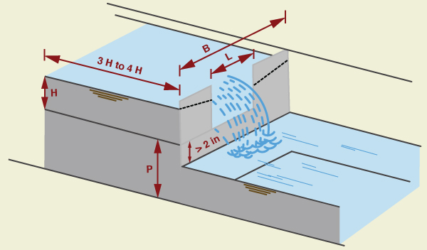
6. The water surface elevation in the downstream channel should be at least 2 in (5 cm, or 0.05 m) below the weir crest (Fig. 4-16).

Gary Player Fig. 4-16  Rectangular weir on Ash Creek, near New Harmony, Utah.

Standard contracted rectangular weir. The standard contracted rectangular weir is shown in Fig. 4-17. To be fully contracted, the overflow plate sides and ends must be located at a distance of at least 2H from the approach flow boundaries. The head is measured at a distance upstream of at least 4H from the weir. The computation procedure follows Section 9 of Chapter 7 of the USBR Water Measurement Manual.

Fig. 4-17  Definition sketch for a standard contracted rectangular weir.

The formula for the standard contracted rectangular weir is the Francis equation. In U.S. Customary units, this equation is:

Q = 3.33 (L - 0.2H ) H 3/2

(4-38)

in which Q = discharge, in cfs, L = length of the weir crest, in ft, and H = head on the weir crest, in ft.

The accuracy of measurements obtained by Eq. 4-38 is considerably less than that obtainable with V-notch weirs. The accuracy of the discharge coefficient is ± 5 percent.

Equation 4-38 has a constant discharge coefficient (3.33), which facilitates computations. However, the coefficient does not remain constant for a ratio of head-to-crest H/L > 1/3, and the actual discharge exceeds that given by the equation. Francis' experiments were made on comparatively long weirs, most of them with crest length L = 10 ft and heads in the range 0.4 ft ≤ H ≤ 1.6 ft. Thus, the equation applies particularly to such conditions. USBR experiments on 6-in, 1-ft, and 2-ft weirs has shown that the Francis equation also applies fairly well to shorter crest lengths L, provided H/L ≤ 1/3.

Equation 4-38 is subject to the following restrictions:

1. Height-to-head ratio P/H ≥ 2.

2. Ratio b/H ≥ 2.

3. Length-to-head ratio:  L/H ≥ 3.

Standard suppressed rectangular weir. A standard suppressed rectangular weir has a horizontal crest that crosses the full channel width (Fig. 4-18). The elevation of the crest is high enough to assure full bottom crest contraction of the nappe. The vertical sidewalls of the approach channel continue downstream past the weir plate, to prevent side contraction or lateral expansion of the overflow jet. The computation procedure follows Section 10 of Chapter 7 of the USBR Water Measurement Manual.

Special care must be taken to secure proper aeration beneath the overflowing sheet at the crest. Aeration is usually accomplished by placing vents on both sides of the weir box under the nappe. Other conditions for accuracy of measurement for this type of weir are generally the same as for those of the contracted rectangular weir, except for the absence of side contraction. However, the crest height P should be at least 3H.

Fig. 4-18  Definition sketch for a standard suppressed rectangular weir.

The formula for the standard suppressed rectangular weir is the Francis equation. In U.S. Customary units, this equation is:

Q = 3.33 (L - 0.2H ) H 3/2

(4-39)

in which Q = discharge, in cfs, L = length of the weir crest, in ft, and H = head on the weir crest, in ft.

The accuracy of the discharge coefficient is ± 5 percent. Equation 4-39 should not be used for heads H < 0.2 ft. These small heads do not give accurate flow measurements because the nappe of water going over the crest may not spring free of the crest.

Equation 4-39 is subject to the following restrictions:

1. Head H ≥ 0.2 ft.

2. Length L ≥ 4 ft.

3. Height-to-head ratio P/H ≥ 3.

4. Length-to-head ratio:  L/H ≥ 3.

The head H is measured at an upstream distance of at least 4H from the weir. The sidewalls must extend a distance of at least 0.3H downstream from the crest. The overflow jet must be adequately ventilated to the atmosphere.

Example 4-4. Using ONLINE STANDARD SUPPRESSED RECTANGULAR, calculate the discharge over a standard suppressed rectangular weir for the following flow conditions: Head H = 0.5 m; length L = 5 m; height P = 2 m.   ONLINE CALCULATION. Using the ONLINE STANDARD SUPPRESSED RECTANGULAR calculator, the discharge is: Q = 3,250 L/s.

QUESTIONS

[Problems]   [References]   •   [Top]   [Critical Flow]   [Computation of Critical Flow]   [Critical Flow Control]   [Sharp-crested Weirs]

1. Why is β, the exponent of the rating, important in open-channel flow?

2. For a given discharge Q, what is the value of specific energy at critical flow?

3. What is the relation between velocity head and hydraulic depth under critical flow?

4. What is the difference bewteen primary and secondary waves in unsteady open-channel flow?

5. How are bottom slope, critical slope, and Froude number related in uniform flow?

6. Why is it extremely rare to have critical or supercritical flow in a natural channel?

7. In a hydraulically wide channel, critical depth is only a function of what hydraulic variable?

8. How many types of control are there in open-channel flow?

9. Under what condition are two gage measurements required in a Parshall flume?

10. Why is full contraction necessary in flow measurement using a sharp-crested weir?

11. Is the Cipolletti weir fully or partially contracted?

12. How is full contraction implemented in a standard suppressed rectangular weir?

PROBLEMS

[References]   •   [Top]   [Critical Flow]   [Computation of Critical Flow]   [Critical Flow Control]   [Sharp-crested Weirs]   [Questions]

1. Using the Chezy equation (Eq. 5-10), derive the formula for the critical slope S_c in a prismatic channel.

2. Using the Manning equation (Eq. 5-17 or Eq. 5-18), derive the formula for the critical slope S_c in a prismatic channel.

3. Calculate the theoretical discharge over a broad-crested weir of length L = 22 ft, when the total head above the weir is H = 1.2 ft. Verify with ONLINE CHANNEL 14.

4. Calculate the theoretical discharge over a broad-crested weir of length L = 8 m, when the total head above the weir is H = 0.5 m. Verify with ONLINE CHANNEL 14.

5. Calculate the critical depth corresponding to a unit-width discharge q = 1.36 m²/s.

6. Given a modified Darcy-Weisbach friction factor f = 0.003 and bottom slope S = 0.002. Calculate the Froude number.

7. Use ONLINE CHANNEL 04 to calculate the critical slope for the following canal data: Q = 11 m³/s, b = 1.5 m, z = 1, S = 0.0006, n = 0.013.

8. Use ONLINE CHANNEL 04 to calculate the critical slope for the following canal data: Q = 35 ft³/s, b = 3 ft, z = 1, S = 0.001, n = 0.015.

9. Use ONLINE CIPOLLETTI to calculate the weir discharge through a Cipolletti weir (Fig. 4-19), given head H = 1 ft, length L = 3.2 ft, height P = 4 ft, and width B = 6 ft.

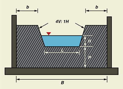
   Fig. 4-19  Definition sketch for a Cipolletti weir.

10. Use ONLINE STANDARD CONTRACTED RECTANGULAR to calculate the weir discharge through a standard contracted rectangular weir (Fig. 4-20), given head H = 0.5 m, length L = 3 m, height P = 3 m, and width b = 1.5 m.

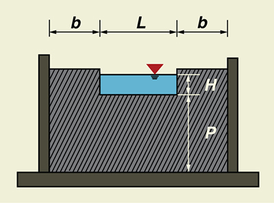
    Fig. 4-20  Definition sketch for a standard contracted rectangular weir.

REFERENCES

•   [Top]   [Critical Flow]   [Computation of Critical Flow]   [Critical Flow Control]   [Sharp-crested Weirs]   [Questions]   [Problems]

Chow, V. T. 1959. Open-channel Hydraulics. McGraw Hill, New York.

Jarrett, R. D., 1984. Hydraulics of High-Gradient Streams. ASCE Journal of Hydraulic Engineering, Vol. 110, No. 11, November, 1519-1539.

Ponce, V, M., and D. B. Simons. 1977. Shallow wave propagation in open-channel flow. Journal of the Hydraulics Division, ASCE, Vol. 103, No. HY12, December, 1461-1476.