|
|
|
CHAPTER 14: HYDROLOGIC DESIGN CRITERIA |
|
"Water will dissolve almost anything to some degree. The dissolved material tends to remain is solution because of water's extreme dielectric constant, which is greater than for any other substance." Howard L. Penman (1970) |
|
This chapter describes selected design criteria and procedures used by U.S. federal agencies. This information is intended to complement the subjects presented in Chapters 4 to 13. |
The techniques of hydrologic analysis described in Chapters 4-13 are useful in hydrologic design and hydrologic forecasting. In hydrologic design, the objective is to predict the behavior of hydrologic variables under a hypothetical extreme condition such as the 100-y flood or the probable maximum flood. In hydrologic forecasting the aim is to predict the behavior of hydrologic variables within a shorter time frame, either daily, monthly, seasonally, or annually. These two types of hydrologic applications are quite different, paralleling the differences between event-driven and continuous-process catchment models (Section 13.1).
Hydrologic design precedes hydraulic design; i.e., the output of hydrologic design is the input to hydraulic design. Hydrologic design determines streamflows, discharges, and headwater levels, from which hydraulic design derives flow depths, velocities, and pressures acting on hydraulic structures and systems. Actual sizing of structures and appurtenances is obtained by balancing efficiency, practicality, and economy.
In practice, hydrologic design translates into hydrologic design criteria, i.e., a set of rules and procedures used by federal, state, or local agencies having cognizance with water resources projects. Of necessity, these criteria are likely to vary widely, reflecting the charter and jurisdiction of each agency, and the size and scope of individual projects.
The following federal agencies are actively engaged in developing and using hydrologic design criteria for engineering applications:
- NOAA National Weather Service
- U.S. Army Corps of Engineers
- USDA Natural Resources Conservation Service
- U.S. Bureau of Reclamation
- U.S. Geological Survey.
14.1 NATIONAL WEATHER SERVICE
|
|
Probable Maximum Precipitation
The Probable Maximum Precipitation (PMP) is the theoretically greatest depth of precipitation for a given duration that is physically possible over a given size storm area, at a particular geographical location, at a certain time of the year [7]. In view of the incomplete knowledge of meteorological processes, calculated PMP values are regarded as estimates [4]. For applications in hydraulic design, a suitable rainfall-runoff transform is used to convert the PMP into the Probable Maximum Flood (PMF).
Estimates of PMP are based on either statistical or deterministic approaches. The statistical approach is based on the analysis of time series. The deterministic approach, commonly referred to as the generalized estimate, is based on regional PMP isoline maps. In the United States, PMP determinations are commonly based on generalized estimates, using isoline maps developed by NOAA National Weather Service. The statistical approach is applicable in regions where a generalized estimate has not been developed.
Statistical Estimates of PMP. The statistical frequency formula is:
xT = x̄n + KT sn
| (14-1) |
in which xT is the rainfall associated with a return period T, x̄n and sn
are the mean and standard deviation of a series of n annual maxima, and KT is the frequency factor
associated with T (
In terms of maximum rainfall, Eq. 14-1 can be expressed as follows:
xM = x̄n + KM sn
| (14-2) |
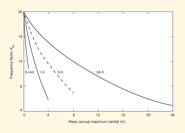
in which xM is the maximum rainfall and KM is the number of standard deviations that must be added to the mean in order to obtain xM.
An empirical estimate of KM may be obtained by enveloping a value of KM based on a large number of computed values. The value KM = 15 was considered initially by Hershfield [1] to be an appropriate enveloping value. This analysis was based on data from 2600 stations, approximately 90% of which were located in the United States. However, Hershfield's later studies [2] have shown that KM actually varies with mean annual maximum rainfall and storm duration, as shown in Fig. 14-1. Note that this procedure gives point estimates of PMP; areal estimates may be obtained through the use of an appropriate depth-area relation.
Figure 14-1 Frequency factor KM as a function of mean annual maximum rainfall and storm duration [2]. |
The step-by-step procedure to estimate the D-hr PMP based on statistical data is the following:
Compile the D-hour annual-maxima rainfall series.
Calculate the mean and standard deviation of the D-hour annual-maxima rainfall series.
Using Fig. 14-1, determine the value of KM as a function of mean annual maximum rainfall and D-hour duration.
Using Eq. 14-2, calculate the D-hour point PMP.
For basins in excess of 25 km2, determine the areal PMP by reducing the point PMP using an appropriate depth-area relation.
Generalized Estimates of PMP. The procedure for determining generalized estimates of PMP varies from nonorographic to orographic regions. For nonorographic regions, the approach consists of performing three operations on observed areal storm precipitation: (1) moisture maximization, (2) transposition, and (3) envelopment. Moisture maximization consists of increasing the storm precipitation to a value that is consistent with the maximum moisture in the atmosphere, for the given storm's geographical location and month of occurrence.
Transposition involves the relocation of storm precipitation within a meteorologically homogeneous region, thereby increasing the quantity of data available for the evaluation of precipitation potential. Envelopment consists of the smooth interpolation between maxima for different durations and areas. In many cases, enveloping curves may increase the values of PMP obtained using only maximization and transposition. Envelopment also produces smooth geographical variations, assuring the consistency of mapped values.
For orographic regions, terrain plays an important role in precipitation, acting both to increase or reduce observed rainfall. Thus, orographic effects from storm-terrain interactions have a bearing on PMP determinations.
In the United States,
the National Oceanic and Atmospheric Administration's (NOAA) National Weather Service (NWS) is
responsible for the development of generalized estimates of probable maximum precipitation (PMP).
The concepts and related methodologies are described in the NOAA NWS Hydrometeorological Report (HMR) series.
Reports of current applicability are listed in
Figure 14-2 Regions covered by HMR reports (Click on the figure to enlarge). |
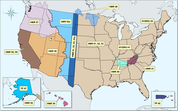
Figure 14-1 shows the following:
HMR 49 applies for the Colorado River and Great Basin drainages.
HMR 51, 52 and 53 apply for regions east of the 105th meridian, i.e., the U.S. East and Midwest, including the central states.
HMR 55A applies for the United States between the Continental Divide and the 103rd meridian (Note the overlap with HMR 51, 52, and 53).
HMR 57 applies for the Pacific Northwest states and Pacific Coastal drainages.
HMR 58 and 59 apply for the state of California.
Other HMR reports apply for smaller regional areas, including Hawaii, Alaska, and Puerto Rico.
PMP Estimates for Regions East of the 105th Meridian.
Procedures for estimating PMP
in
Figure 14-3 All-season PMP (in.) for 24-h 10-mi2 rainfall (Click on the figure to enlarge) [4]. |
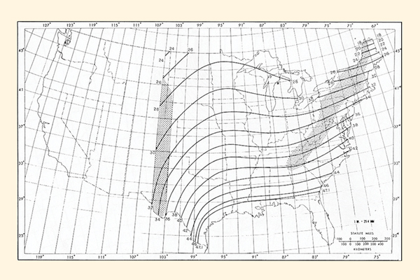
Generalized PMP estimates can be obtained by the following steps, as explained in HMR 51 [4]:
Determine the geographical location and area of the drainage basin under study.
Using the maps in HMR 51, prepare a table of PMP depths applicable to the given geographical location. Use the maps of all five (5) durations and of at least four (4) areas comprising the drainage basin size of interest. For instance, for a basin size of 11,300 mi2, tabulate 5 × 4 =
20 PMP depths (obtained from the 6-, 12-, 24-, 48-, and 72-hr maps, and from the 1000-, 5000-, 10,000-, and 20,000-mi2 area maps).For each of five (5) durations (6-, 12-, 24-, 48-, and 72-hr), plot PMP depths versus basin area on semilogarithmic paper, with PMP depth in the abscissas (arithmetic scale) and basin area in the ordinates (logarithmic scale), to obtain a PMP depth-area-duration (DAD) relation.
Using the PMP DAD relation developed in step 3, determine, for the given basin area, the applicable PMP depth for each of five (5) durations.
Plot PMP depth versus duration on arithmetic scales and draw a smooth curve connecting these points, to determine the PMP depth-duration relation for the given basin area size and geographical location.
Determine the 6-h incremental PMP depths using the PMP depth-duration relation developed in step 5. The 6-h incremental PMP is the PMP expressed in 6-h increments. This is accomplished by calculating the PMP depth for successive durations in multiples of 6 h, and subtracting two consecutive PMP depths to determine an incremental PMP value. For instance, the difference between the 24- and 18-h PMP depth is the 6-h incremental PMP depth associated with the 18- to 24-h time interval.
The application of HMR 51 to specific drainage basins, including the temporal and spatial distribution of the probable maximum storm is described in HMR 52 [5].
PMP Estimates for Regions West of the Continental Divide. The procedures for estimating PMP for U.S. regions west of the Continental Divide are described in the following HMR reports:
HMR 49: Colorado River and Great Basin drainages [3],
HMR 57: Pacific Northwest States) [8], and
HMR 58 and HMR 59: California [9, 10].
Unlike the case of the U.S. regions east of the 105th meridian, in regions west of the Continental Divide, the local storm (thunderstorm) is not enveloped with general-storm depth-duration data.
The estimates of local-storm PMP comprise durations varying from 15 minutes to 6 hours, and drainage areas between 1 and 500 mi2 (2.59 and 1,295 km2). Local-storm PMP is applicable to the warm season, between May and October.
PMP Estimates for California.
The procedures for estimating PMP in California are
described in HMR 58 and HMR 59 [9, 10]. Note that HMR 58 is contained in HMR 59.
HMR 58 provides estimates of general-storm PMP for a given drainage area, for durations
of
In HMR 58, the local-storm PMP comprises durations varying from 15 minutes to 6 hours, and drainage areas between 1 and 500 mi2 (2.59 and 1,295 km2). For basins less than 500 mi2, it is necessary to calculate both general- and local-storm PMP. The larger of these estimates is the applicable PMP for the given basin.
General-Storm PMP Computation for California. The procedure for estimating a general-storm all-season PMP in California is the following:
Basin location
Find the geographical location of the basin of interest.
Evaluate the basin outline and its drainage area.
All-season PMP index estimate [10-mi2 24-h ]
Overlay the drainage area on the appropriate general-storm PMP index map.
Two maps are provided in HMR 59 [10]: California-South, also shown here asFig. 14-4 (a); and California-North, also shown here asFig. 14-4 (b). Cover the entire drainage area with a uniform grid.
Determine the average general-storm PMP index [10-mi2 24-h] applicable to the entire drainage area.
Depth-duration ratios and 10-mi2 PMP depths
Locate the basin within one of the regions of California shown in Fig. 14-5. Note that occasionally the basin may subtend more than one region.
Use Table 14-2 to determine the appropriate all-season PMP depth-duration ratios. Use proportionally region-weighted values if more than one subregion is subtended by the basin.
Multiply the depth-duration ratios (obtained in Step 3b) by the average general-storm PMP index [10-mi2 24-h] (obtained in Step 2c) to calculate 10-mi2 PMP depths for durations of 1, 6, 12, 24, 48, and 72 h.
Table 14-2. California all-season PMP depth-duration ratios.* No. Region Duration (h) 1 6 12 24 12 24 1 Northwest 0.10 0.40 0.73 1.00 1.49 1.77 2 Northeast 0.16 0.52 0.69 1.00 1.40 1.55 3 Midcoastal 0.13 0.45 0.74 1.00 1.45 1.70 4 Central Valley 0.13 0.42 0.65 1.00 1.48 1.75 5 Sierra 0.14 0.42 0.65 1.00 1.56 1.76 6 Southwest 0.14 0.48 0.76 1.00 1.41 1.59 7 Southeast 0.30 0.60 0.86 1.00 1.17 1.28 * This table is the same as Table 2.1 of HMR 58. Areal reduction factors
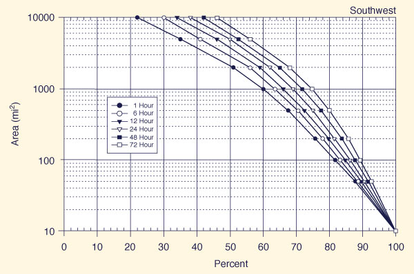
With the appropriate region known (Fig. 14-5), use one of Figs. 14-6 (a) to 14-6 (f) t obtain, for each of six (6) storm durations (1, 6, 12, 24, 48, and 72 h), the applicable all-season percent areal reduction.
Multiply the PMP depths (calculated in Step 3c) by the percent areal reductions (obtained in Step 4a) and divide by 100 to obtain the area-reduced PMP depths.
Incremental PMP values
Plot the results of Step 4b on an arithmetic graph and draw a smooth curve.
Obtain cumulative 6-h PMP values.
Each discrete 6-h PMP incremental value is the difference between two consecutive cumulative values.
Temporal distribution of PMP
To provide the most critical 72-h PMP storm sequence, group the four heaviest 6-h incremental values in a 24-h sequence, as follows:
Place the second highest value next to the highest, to provide the most critical 12-h sequence;
Place the third highest on either side of the 12-h sequence, to provide the most critical 18-h sequence, and
Place the fourth highest on either side of the 18-h sequence.
The 24-h heaviest sequence may be positioned anywhere in the 72-h period. The remaining eight 6-h amounts may be positioned anywhere else. For PMF purposes, critical PMP sequences are usually obtained by trial and error.
Spatial distribution of PMP
There are no fixed rules to develop a spatial storm pattern for general-storm PMP determinations. In the absence of local data, established NOAA National Weather Service isopercental curves may be used.
A spatial storm pattern for PMP may also be based on a significant storm with a sufficient number of observations. However, only a few California storms have sufficient detail to define a storm pattern.
Figure 14-4 (a)
General-storm PMP Index map for California - South |
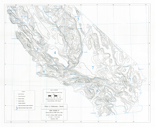
Figure 14-4 (b)
General-storm PMP Index map for California - North |
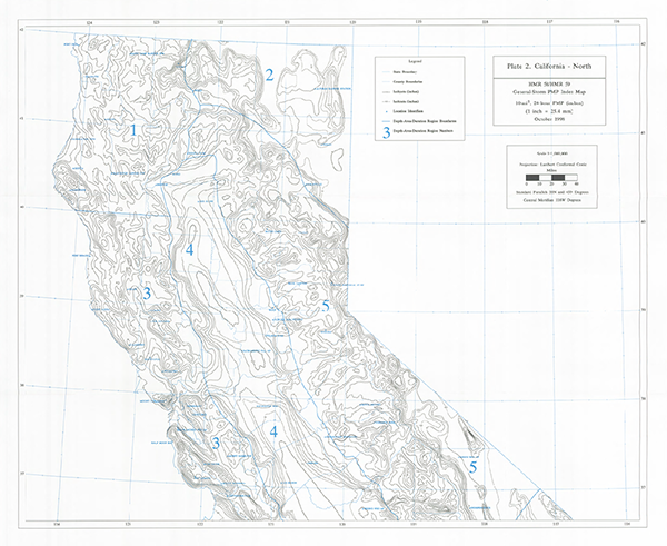
Figure 14-5
Regional boundaries for the development of depth-duration ratios in California |

Figure 14-6 (a)
Depth-area-duration relation for the Northwest-Northeast region of California |
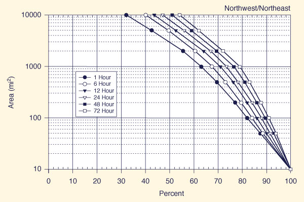
Figure 14-6 (b)
Depth-area-duration relation for the Midcoastal region of California |
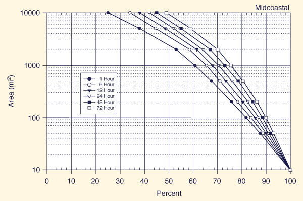
Figure 14-6 (c)
Depth-area-duration relation for the Central Valley region of California |
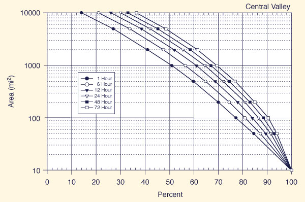
Figure 14-6 (d)
Depth-area-duration relation for the Sierra region of California |
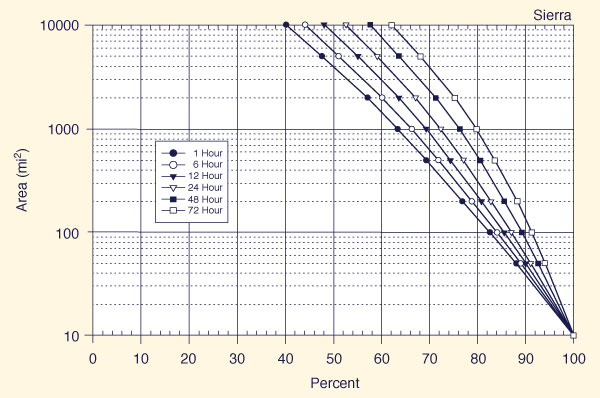
Figure 14-6 (e)
Depth-area-duration relation for the Southeast region of California |
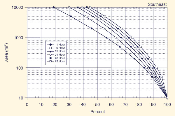
Figure 14-6 (f)
Depth-area-duration relation for the Southwest region of California |
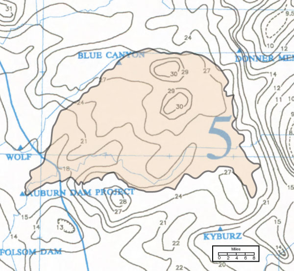
Example of General-Storm PMP Computation for California. The Auburn Dam drainage basin above Folsom Lake, California, is used as an example of a general-storm PMP computation. This example is described in HMR 58 [9] (Fig. 14-7).
Figure 14-7
Delineation of Auburn dam drainage basin on the general-storm PMP index map |
The following steps are used to calculate the all-season PMP:
Basin location
The basin is located in Region 5 Sierra of California-North PMP index map, as shown in Fig. 14-5.
The drainage area is 973 mi2.
All-season PMP index estimate [10-mi2 24-h]
The average general-storm PMP index within the drainage area shown in Fig. 14-7 is calculated to be equal to
24.6 mi2. Depth-duration ratios and 10-mi2 PMP depths
The Auburn drainage basin is within Region 5 (Sierra), except for a very small portion near the damsite, which may be regarded as inconsequential (Fig. 14-5). Table 14-3 shows the applicable depth-duration ratios, extracted from Table 14-2.
Table 14-3. All-season PMP depth-duration ratios for the Sierra region. No. Region Duration (h) 1 6 12 24 12 24 5 Sierra 0.14 0.42 0.65 1.00 1.56 1.76 Table 14-4 shows the all-season 10-mi2 PMP depths, obtained by multiplying the average
[10 mi2 24-h] PMP index value of 24.6 in (obtained in Step 2) times each one of the depth-duration ratios shown in Table 14-3.Table 14-4. All-season 10-mi2 PMP depths (in) for the Auburn drainage. No. Region Duration (h) 1 6 12 24 12 24 5 Sierra 3.44 10.3 16.0 24.6 38.4 43.3 -
Areal reduction factors
Use Fig. 14-6 (d) (Sierra) to determine all-season areal reduction factors for each of six (6) storm durations: 1, 6, 12, 24, 48, and 72 h. The areal reduction factors are shown in Table 14-5.
Table 14-5. All-season areal reduction factors for the Auburn drainage. Drainage area
(mi2)Duration (h) 1 6 12 24 12 24 973 0.64 0.67 0.70 0.72 0.77 0.80 Multiply the all-season 10-mi2 PMP depths shown in Table 14-4 times the corresponding area reduction factors shown in Table 14-5 to obtain the all-season PMP depth-duration results shown in Table 14-6.
Table 14-6. All-season PMP depth-duration for the Auburn drainage. Duration (h) 1 6 12 24 12 24 PMP depth (in) 2.2 6.9 11.2 17.7 29.6 34.6 Incremental PMP values
Figure 14-8 shows depth-duration curves for the all-season PMP depths shown in
Table 14-6. The All-season PMP is shown as a solid line. Also shown in the seasonal PMP (May), calculated in the seasonal PMP section (next section).Table 14-7 shows the 6-h cumulative all-season PMP depths obtained from Fig. 14-7.
Table 14-8 shows the 6-h incremental all-season PMP depths obtained from Table 14-7.Table 14-7. 6-h cumulative all-season PMP depths for the Auburn drainage. Duration (h) 6 12 18 24 30 36 42 48 54 60 66 72 PMP (in) 6.9 11.2 14.6 17.7 20.8 23.8 26.7 29.6 31.6 32.7 33.7 34.6 Table 14-8. 6-h incremental all-season PMP depths for the Auburn drainage. Duration (h) 6 12 18 24 30 36 42 48 54 60 66 72 PMP (in) 6.9 4.3 3.4 3.1 3.1 3.0 2.9 2.9 2.0 1.1 1.0 0.9 Temporal distribution of PMP
Using the rules for temporal distribution of PMP, a possible 72-h storm sequence, in 6-h increments, is selected. Table 14-9 shows the chosen sequence.
Table 14-9. Possible all-season 72-h PMP storm for the Auburn drainage, in 6-h increments. Duration (h) 6 12 18 24 30 36 42 48 54 60 66 72 PMP (in) 3.1 3.0 2.9 2.9 3.1 4.3 6.9 3.4 1.1 0.9 2.0 1.0
Figure 14-8 Depth-duration curves for the Auburn dam drainage basin (Click on the figure to enlarge) [9]. |

Example of Seasonal-Storm PMP Computation for California. The following example describes a seasonal-storm PMP computation for California. The procedure is for the month of May for the Auburn drainage (Fig. 14-7).
The all-season PMP index value, calculated in the previous section, is 24.6 in.
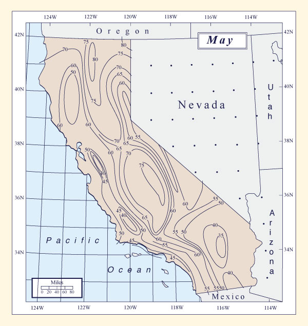
Figure 14-9 shows
the variation of general-storm PMP for the month of May, as a percent of all-season PMP.
By placing the Auburn drainage (Fig. 14-7) in its geographical location in Fig. 14-9, a value of 68% for the Auburn drainage is obtained (See
Note below).
Therefore,
the average PMP depth for the Auburn drainage for the month of May is:
Note: A complete set of 10-mi2 general-storm PMP for each month of the year, as a percent of all-season PMP, is given in |
Figure 14-9 10-mi2 24-h general-storm PMP for the month of May, as a percent |
Examination of the general-storm monthly PMP maps shows that the nearest all-season month
for the Auburn drainage location is March, and the monthly offset is 2 (May to March, i.e., two-months difference).
Table 14-10 shows the seasonally adjusted 2-month-offset
|
Table 14-10. Seasonally adjusted 2-month-offset 10-mi2 PMP depth-duration ratios for the Sierra region.* | ||||||||
| No. | Region | Offset (months) |
Duration (h) | |||||
| 1 | 6 | 12 | 24 | 12 | 24 | |||
| 5 | Sierra | 2 | 0.148 | 0.437 | 0.663 | 1.000 | 1.451 | 1.549 |
|
* These values were obtained from the appropriate line of
|
||||||||
Table 14-11 shows the seasonally adjusted May 10-mi2 PMP,
obtained by multiplying the calculated PMP depth for the month of May (16.7 in) by each one of the depth-duration ratios shown in
| Table 14-11. Seasonally adjusted May 10-mi2 PMP for the Auburn drainage. | ||||||||
| No. | Region | Offset (months) |
Duration (h) | |||||
| 1 | 6 | 12 | 24 | 12 | 24 | |||
| 5 | Sierra | 2 | 2.5 | 7.3 | 11.1 | 16.7 | 24.2 | 25.9 |
Table 14-12 shows the seasonally adjusted areal reduction factors for the Sierra region, 2-month offset.
|
Table 14-12. Seasonally adjusted areal reduction factors for the Auburn drainage, 2-month offset.* | |||||||
| Drainage area
(mi2) |
Duration (h) | ||||||
| 1 | 6 | 12 | 24 | 12 | 24 | ||
| 973 | 0.548 | 0.607 | 0.648 | 0.687 | 0.731 | 0.773 | |
| * These values were obtained from the appropriate line of Table 2.7 of HMR 58, by interpolation to 973 mi2. The complete set of tables of seasonally adjusted areal reduction factors is given in Tables 2.4 to 2.9 of HMR 58. | |||||||
Table 14-13 shows the seasonally adjusted May PMP for the Auburn drainage, obtained by multiplying the seasonally adjusted May 10-mi2 PMP values shown in Table 14-11
times the corresponding areal reduction factors shown in
| Table 14-13. Seasonally adjusted May PMP depth-duration for the Auburn drainage. | ||||||
| Duration (h) | 1 | 6 | 12 | 24 | 12 | 24 |
| PMP depth (in) | 1.4 | 4.4 | 7.2 | 11.5 | 17.7 | 20.0 |
The seasonally adjusted May PMP depth-duration results shown in Table 14-13 are plotted in
|
Table 14-14. 6-h cumulative seasonally adjusted (May) PMP depths for the Auburn drainage. | ||||||||||||
| Duration (h) | 6 | 12 | 18 | 24 | 30 | 36 | 42 | 48 | 54 | 60 | 66 | 72 |
| PMP (in) | 4.4 | 7.2 | 9.4 | 11.5 | 13.3 | 15.0 | 16.4 | 17.7 | 18.5 | 19.1 | 19.6 | 20.0 |
Table 14-15 shows the 6-h incremental seasonally adjusted (May) PMP depths obtained from Table 14-14.
| Table 14-15. 6-h incremental seasonally adjusted (May) PMP depths for the Auburn drainage. | ||||||||||||
| Duration (h) | 6 | 12 | 18 | 24 | 30 | 36 | 42 | 48 | 54 | 60 | 66 | 72 |
| PMP (in) | 4.4 | 2.8 | 2.2 | 2.1 | 1.8 | 1.7 | 1.4 | 1.3 | 0.8 | 0.6 | 0.5 | 0.4 |
Using the rules for temporal distribution of PMP, a possible 72-h storm sequence, in 6-h increments, is selected. Table 14-16 shows the chosen sequence.
| Table 14-16. Possible seasonally adjusted (May) 72-h PMP storm for the Auburn drainage, in 6-h increments. | ||||||||||||
| Duration (h) | 6 | 12 | 18 | 24 | 30 | 36 | 42 | 48 | 54 | 60 | 66 | 72 |
| PMP (in) | 0.6 | 0.8 | 2.2 | 4.4 | 2.8 | 2.1 | 1.8 | 1.7 | 1.4 | 1.3 | 0.5 | 0.4 |
Local-Storm PMP Computation for California. There are two procedures to calculate the local-storm PMP for California:
Average depth, and
Spatially distributed depth.
The PMP calculated using the average-depth method is usually greater than that calculated using the spatially distributed method.
The following steps are used to calculate the local-storm PMP:
1-h 1-mi2 local-storm PMP index
Determine a 1-h 1-mi2 local-storm PMP index by overlaying the watershed of interest on the map shown in
Fig. 14-10. Use linear interpolation.
Mean basin elevation adjustment
Determine the mean basin elevation. No adjustment is necessary for elevations less than or equal to 6,000 ft.
For elevations greater than 6,000 ft, reduce the PMP index depth obtained in Step 1a by 9% for every 1,000 ft above the 6,000 ft threshold. For example, for the elevation of 8,700 ft, the adjustment is: [(8,700 - 6,000)/1000] × 9% = 24.3%, rounded to 24%. Therefore, the elevation-adjusted PMP is: PMP ×
(100 - 24)/100 = (0.76) PMP.
Storm duration adjustment
The 1-mi2 local-storm PMP for durations less than 1 hour are obtained from Fig. 14-11 as a percentage of the 1-h 1-mi2 local-storm PMP index obtained in Step 1a.
The 1-mi2 local storm PMP for durations greater than 1 h is calculated as follows:
Locate the basin in Fig. 14-12 and determine the ratio of 6-h to 1-h local-storm PMP from the map, for example 1.15;
The values shown in Fig. 14-12 are labeled type curve A (1.15), B (1.2), C (1.3), or D (1.4);
Enter Fig. 14-11 for the chosen type curve (A, B, C, or D) to obtain the percentage of the 1-h 1-mi2 local-storm PMP index for durations greater than 1 h, up to 6 h.
-
Areal reduction factors
Figure 14-13 shows the California 1-mi2 local-storm depth-area relation for a 6-h to 1-h depth-duration adjustment ratio less than 1.2 (< 1.2). If this is the case, enter Fig. 14-13 with the basin area in the abscissas to the curve for the respective duration (1/4-h to 6-h) to determine the percent of 1-mi2 depth in the ordinates.
A complete set of California 1-mi2 local-storm depth-area relations for all four values of 6-h to 1-h depth-duration adjustment ratios (< 1.2, 1.2, 1.3, and 1.4) is given in California local-storm depth-area relations.
Temporal storm distribution
The review of local-storm temporal distributions for California shows that most storms have durations less than 6 h and that the greatest 1-h amount occurs in the first hour. The recommended sequence of hourly increments is as follows:
Obtain the hourly increments by successive subtraction from the smoothed depth-duration curve (Fig. 4-10) or from Table 4-17.
Arrange the hourly increments from largest to smallest: the most intense 1-h increment occurs in the first hour, the second most intense occurs in the second hour, and so forth.
Table 14-17. Depth-duration relations (in percent of 1-h amounts)
applicable to 1-mi2 local-storm PMP in California.Duration
(h)A B C D 0 0 0 0 0 1/4 55 55 55 55 1/2 79 79 79 79 3/4 91 91 91 91 1 100 100 100 100 2 109.5 110.5 114 117 3 112 116 120 126 4 114 118 125 132 5 114.5 119 128 137 6 115 120 130 140 Areal distribution of local-storm PMP
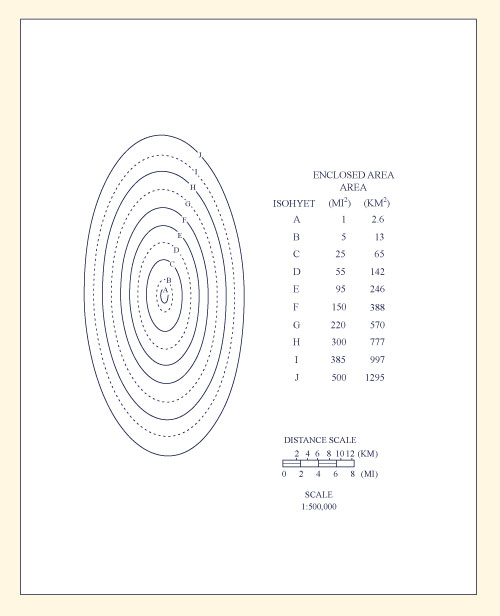
Figure 4-14 shows an idealized isohyetal pattern for local-storm PMP areas up to 500-mi2. The elliptical lettered pattern (A-J) of Fig. 4-13 and the tabulated percentages in
HMR 58 Table 2.11 (ratio < 1.2),Table 2.12 (ratio = 1.2), Table 2.13 (ratio = 1.3), andTable 2.14 (ratio = 1.4) are used to describe the areal distribution of precipitation of a local-storm PMP. [These HMR 58 tables are given in HMR 58 local-storm areal distribution tables].The 2:1 ratio of the major to minor axis of Fig. 14-14 should be placed only on a map at 1:500,000 scale.
The average index value from Step 2a or 2b is multiplied times each of the percentages from the appropriate HRM 58 local-storm areal distribution tables to obtain the value for each lettered isohyet (A-J).
Once the labels have been determined for each application, the pattern can be moved to different placements on the basin.
In most instance, the greatest volume of precipitation will be obtained when the pattern is centered in the drainage. However, peak flows may actually occur with placements closer to the drainage outlet.
Figure 14-10 California 1-h 1-mi2 local-storm PMP index map |
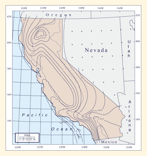
Figure 14-11 California 1-mi2 local-storm depth-duration relations |
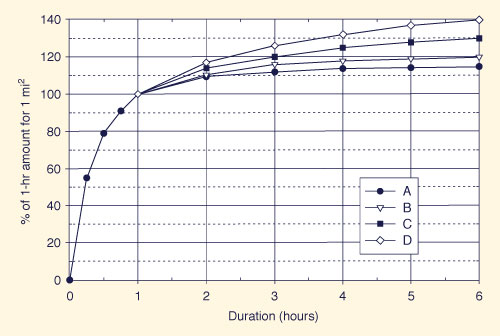
Figure 14-12 California 1-mi2 local-storm depth-duration adjustment ratios |
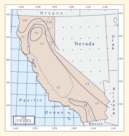
Figure 14-13 California 1-mi2 local-storm depth-area relation |
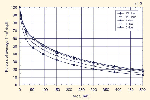
Figure 14-14 Idealized isohyetal pattern for local-storm PMP for areas up to 500-mi2 |
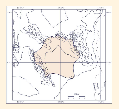
Example of Local-Storm PMP Computation for California. An example of local-storm PMP computation is described here. The selected basin is McCoy Wash, a small 176-mi2 drainage located in southeastern California. This example is taken from HMR 58 [9].
Figure 14-15 shows the geographical location of the basin. Superposition of the basin outline on
Figure 14-15 Drainage area of McCoy Wash,
in Southeastern California, with elevation contours |
From Fig. 14-12, the applicable adjustment ratio for the given geographical location is 1.3 (curve C in Fig. 14-11). Table 14-18 shows the depth-duration adjustment ratios and the corresponding local-storm 1-mi2 PMP values adjusted for duration.
| Table 14-18. 1-mi2 local-storm PMP depth-duration for the McCoy Wash drainage. | |||||||||
|
Duration (h) |
1/4 | 1/2 | 3/4 | 1 | 2 | 3 | 4 | 5 | 6 |
| Adjustment ratio * | 0.55 | 0.79 | 0.91 | 1.00 | 1.14 | 1.20 | 1.25 | 1.28 | 1.30 |
| PMP (in) |
6.3 | 9.0 | 10.4 | 11.4 | 13.0 | 13.7 | 14.3 | 14.6 | 14.8 |
| * These values correspond to those of curve C, Fig. 14-10. | |||||||||
Figure 2-27 of HMR 58 (California local-storm depth-area relations) shows the depth-area relations for a California local-storm PMP for a 1-mi2 6-h to 1-h depth-duration adjustment ratio equal to 1.3 (curve C).
Table 14-19 shows the area-reduced 167-mi2 local-storm PMP depth-duration for the McCoy Wash drainage.
For each duration, the PMP values shown in
Table 14-19 were obtained by multiplying the corresponding PMP value of Table 14-18 (for instance, 11.4 for 1 h) times
the
(percent of 1-mi2)/100 (that is, 0.43 for 1 h) shown in Table 14-19.
Thus, for 1-h duration, the local-storm 167-mi2 PMP is:
| Table 14-19. 167-mi2 local-storm PMP depth-duration for the McCoy Wash drainage. | |||||||||
| Duration (h) | 1/4 | 1/2 | 1 | 3 | 6 | ||||
| (Percent of 1-mi2) /100 * | 0.31 | 0.37 | 0.43 | 0.50 | 0.54 | ||||
| PMP (in) | 2.0 | 3.3 | 4.9 | 6.9 | 8.0 | ||||
| * These values are taken from Fig 2-27 [HMR 58] by interpolation to 167-mi2. | |||||||||
Figure 14-16 Average depth of local-storm PMP
for the 167-mi2 McCoy Wash, California |
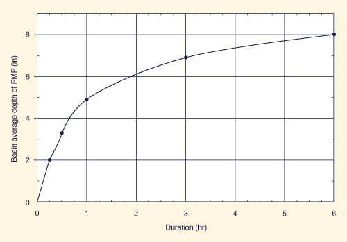
Table 14-20 shows the 167-mi2 local-storm PMP for the McCoy Wash drainage. The cumulative PMP values are obtained from Fig. 14-16 at every hourly interval. The incremental PMP values are obtained by successive subtraction of the respective cumulative values. The highest-to-lowest increment sequence shown in Table 14-20 is the recommended one for the local-storm PMP.
| Table 14-20. 167-mi2 local-storm PMP for the McCoy Wash drainage. | ||||||
| Duration (h) | 1 | 2 | 3 | 4 | 5 | 6 |
| Cumulative PMP (in) | 4.9 | 6.1 | 6.9 | 7.4 | 7.7 | 8.0 |
| Incremental PMP (in) | 4.9 | 1.2 | 0.8 | 0.5 | 0.3 | 0.3 |
The areal distribution of PMP isohyets is shown in Fig. 14-14.
This elliptical lettered pattern (A-J) comprises an area of 500 mi2, at a scale of
1:500,000. For this example (McCoy Wash), the percentages
from Table 2.13 of HMR 58 apply, i.e., for a basin with a
6-h to 1-h ratio of 1.3 (curve C).
For completeness, Table 2-13 of HMR 58
is repeated here as
| Table 14-21. Isohyetal label values,
in percent of 1-mi2 1-h local-storm PMP, corresponding to curve C of Fig. 14-10. | ||||||||||
|
Isohyetal tag |
Area (mi2) |
Duration (h) | ||||||||
| 1/4 | 1/2 | 3/4 | 1 | 2 | 3 | 4 | 5 | 6 | ||
| A | 1 | 55 | 79 | 91 | 100 | 114 | 120 | 125 | 128 | 130 |
| B | 5 | 44 | 66 | 77.6 | 86 | 100 | 106 | 111 | 114 | 116 |
| C | 25 | 26 | 44 | 53.6 | 61 | 74 | 81 | 86 | 89 | 91 |
| D | 55 | 17 | 31 | 40.2 | 46.5 | 58 | 65 | 70 | 73 | 75 |
| E | 95 | 11 | 20 | 26.8 | 32.5 | 42 | 49 | 54 | 57 | 59 |
| F | 150 | 6.6 | 13 | 19 | 24 | 32 | 38 | 43 | 46 | 48 |
| G | 220 | 6.5 | 11 | 14 | 16 | 23 | 28 | 33 | 36 | 38 |
| H | 300 | 5 | 8 | 10.5 | 12 | 17.5 | 21.5 | 25.5 | 29 | 31 |
| I | 385 | 3 | 6 | 8.5 | 10.5 | 16 | 20 | 24 | 27.5 | 30 |
| J | 500 | 2.5 | 5.5 | 8 | 10 | 15 | 19 | 23 | 26.5 | 29 |
Table 14-22 shows the isohyetal label values for local-storm PMP for the McCoy drainage. Values in this table were obtained by multiplying 11.4 in, corresponding to the 1-mi2 1-h PMP depth, times each one of the values of Table 14-21.
For comparison, the spatially averaged 6-h PMP for the 167-mi2 McCoy Wash is 8 in (Table 14-19).
On the other hand, from Table 14-22, for a 6-h PMP, the isohyetal labels range from 14.82 inches
| Table 14-22. Isohyetal label values for local-storm PMP for the McCoy Wash drainage (167 mi2). | ||||||||||
|
Isohyetal tag |
Area (mi2) |
Duration (h) | ||||||||
| 1/4 | 1/2 | 3/4 | 1 | 2 | 3 | 4 | 5 | 6 | ||
| A | 1 | 6.27 | 9.01 | 10.37 | 11.40 | 13.00 | 13.68 | 14.25 | 14.59 | 14.82 |
| B | 5 | 5.02 | 7.52 | 8.85 | 9.80 | 11.40 | 12.08 | 12.65 | 13.00 | 13.22 |
| C | 25 | 2.96 | 5.02 | 6.11 | 6.95 | 8.44 | 9.23 | 9.80 | 10.15 | 10.37 |
| D | 55 | 1.94 | 3.53 | 4.58 | 5.30 | 6.61 | 7.41 | 7.98 | 8.32 | 8.55 |
| E | 95 | 1.25 | 2.28 | 3.06 | 3.71 | 4.79 | 5.59 | 6.16 | 6.50 | 6.72 |
| F | 150 | 0.75 | 1.48 | 2.17 | 2.74 | 3.65 | 4.33 | 4.90 | 5.24 | 5.47 |
| G | 220 | 0.74 | 1.25 | 1.60 | 1.82 | 2.62 | 3.19 | 3.76 | 4.10 | 4.33 |
| H | 300 | 0.57 | 0.91 | 1.20 | 1.37 | 2.00 | 2.45 | 2.91 | 3.31 | 3.53 |
| I | 385 | 0.34 | 0.68 | 0.97 | 1.20 | 1.82 | 2.28 | 2.74 | 3.14 | 3.42 |
| J | 500 | 0.29 | 0.63 | 0.91 | 1.14 | 1.71 | 2.17 | 2.62 | 3.02 | 3.31 |
Note that the isohyetal storm pattern of Fig. 14-14 will produce the spatially averaged PMP depth only if the basin under consideration is of elliptical shape, with a 2:1 ratio of the major to minor axis, and the ellipses are centered in a "perfect" drainage. When placed on an irregularly shaped drainage, the isohyetal storm pattern of Fig. 14-14 will produce an average depth which is less than the spatially averaged PMP depth. In this case, the spatially averaged PMP depth should be used, and the isohyetal pattern is interpreted as a guide to a possible spatial distribution of the local-storm PMP.
NWS Depth-Area Reduction Criteria
Several rainfall atlases containing isopluvial maps, applicable for storm durations up to 10 d, frequencies up to 100 y, and drainage areas up to 400 mi2, have been published by the National Weather Service (see Table 13-1). These maps were developed by analyzing extensive point-rainfall measurements and, therefore, rainfall depths shown represent point-rainfall values.
Each atlas contains a chart of depth-area ratios designed to account for spatial averaging of rainfall depth with increasing basin area. These depth-area ratios allow the calculation of an areally averaged rainfall depth, given the basin area, storm duration, and point depth obtained from the appropriate isopluvial map. These ratios are referred to as geographically fixed depth-area ratios in order to distinguish them from storm-centered depth-area ratios, which are based on the morphological characteristics of individual storms [39].
Traditionally, the development of geographically fixed depth-area ratios has been based on empirical comparisons of point and areal rainfall at the same geographic location. Areal rainfall is approximated by averaging simultaneous gage measurements. This requirement of simultaneity limits the amount of usable data to that of recording gages. Therefore, depth-area ratios are developed based on data from a few existing networks of densely placed recording gages. Due to the sparseness of data, durational, frequency, and geographic variations of depth-area ratios cannot be readily ascertained. Therefore, the available data have been condensed into a single graph (based on a 2-y return period) applicable for depth-area reductions across the United States and for return periods up to 100 y. This graph, reproduced from NOAA Atlas 2 [31], is shown in Fig. 2-13 (a).
A general methodology to compute regional depth-area ratios has been developed by the National Weather Service. In this method, the depth-area ratios are computed using the mean and standard deviations of the annual series of rainfall averages over circular areas. The method is summarized by the following formula:
x' (D, A, n) + K (T, n) s' (D, A, n) Cv (D) DA (T, D, A) = ____________________________________________ 1 + K (T, n) Cv (D)
| (14-3) |
in which DA = depth-area ratio; x' = relative mean; K = Gumbel frequency factor normalized for a 20-y record length; s' = relative standard deviation; Cv = variance coefficient; and A, D, n and T are area, duration, record length, and return period, respectively. The statistics used in Eq. 14-3 are obtained using procedures described in [32].
A depth-area reduction chart for Chicago based on Eq. 14-3 is shown in Fig. 14-17. The close resemblance between Figs. 2-13 (a) and 14-17 is attributed to the fact that the Chicago data had a prominent role in the development of Fig. 2-13 (a). Other geographic regions are likely to have different depth-area ratio patterns.
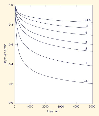
Figure 14-17 (a) and (b) shows depth-area ratios decreasing with increasing area and return period, and decreasing with duration. The effect of return period on depth-area ratio is not accounted for by Fig. 2-13 (a). In addition, Eq. 14-3 can be used to develop depth-area ratios for areas larger than those depicted in Fig. 2-13 (a). For example, a depth-area reduction chart for Chicago, applicable to areas up to 5000 mi2, is shown in Fig. 14-18.
Figure 14-17 (a) 2-y depth-area ratios for Chicago, Illinois [32]. |
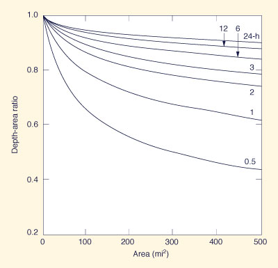
Figure 14-17 (b) 100-y depth-area ratios for Chicago, Illinois [32]. |
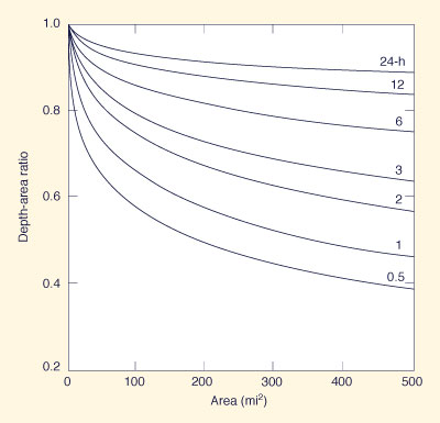
Figure 14-18 2-y depth-area ratios for Chicago, Illinois, for areas up to 5,000 mi2 [32]. |
14.2 ARMY CORPS OF ENGINEERS
|
|
Standard Project Flood Determinations
Hydrologic design criteria used by the U.S. Army Corps of Engineers are outlined in Civil Engineer Bulletin No. 52-8: "Standard Project Flood Determinations," revised March 1965 [45]. A standard project storm (SPS) for a particular drainage area and season of the year is the most severe flood-producing rainfall depth-area-duration relationship and related isohyetal pattern that is reasonably characteristic for the region. The standard project flood (SPF) is the flood hydrograph derived from the SPS. For areas where snowmelt may contribute a substantial volume to runoff, appropriate allowances are made to increase the value of the SPS. When floods are primarily caused by snowmelt, the calculation of SPF is based on estimates of the most critical combination of snow, temperature, and hydrologic abstractions.
Type of Flood Estimates. Flood magnitudes are governed by a combination of several factors, among them, the quantity, intensity, temporal, and spatial distribution of precipitation, the infiltration capacity of the soil mantle, and the natural and artificial storage effects. When relatively long periods of streamflow records are available, statistical analyses can be used to develop flood estimates associated with frequencies bearing a reasonable relationship to the record length. However, for large projects, it is necessary to supplement statistical methods with hypothetical design flood estimates based on rainfall-runoff analysis.
Three types of flood estimates are used in flood-control planning and design investigations:
Statistical analysis of streamflow records, including individual-station flood-frequency estimates and regional flood-frequency analysis.
SPF estimates, which represent flood discharges that are expected to be caused by the most severe combination of meteorologic and hydrologic conditions that are considered to be reasonably characteristic of the region, excluding extremely rare combinations.
PMF estimates, which represent flood discharges that are expected to be caused by the most severe combination of critical meteorologic and hydrologic conditions that are reasonably possible in the region.
Statistical flood determinations are useful in project investigations, primarily as a basis for estimating the mean annual benefits that may be expected to accrue from the control or reduction of floods of relatively common occurrence.
An SPF serves the following purposes: (1) it represents a standard against which the selected degree of protection may be judged and compared with the protection provided at similar projects in different localities and (2) it represents the flood discharge that should be selected as the design flood for the project, where some small risk can be tolerated, but where an unusually high degree of protection is justified because of the risk to life and property.
A PMF is applicable to projects calling for a virtual elimination of the risk of failure. PMF applications are typically in the sizing of spillways for large dams or dams located immediately upstream of heavily populated areas.
Design Flood. The term design flood refers to the flood hydrograph or peak discharge value that is finally adopted as the basis for engineering design, after giving due consideration to flood characteristics, flood frequency, and flood damage potential, including economic and other related factors.
The selected design flood may be either greater or smaller than the SPF. However, in Corps of Engineers' practice, the SPF is intended to be a practical expression of the degree of protection sought in the design of flood control works. Since SPF estimates are based on generalized studies of meteorologic and hydrologic conditions, they provide a basis for comparing the degree of protection afforded by projects in different localities.
Generalized SPS Estimates for Small Basins. The procedures for obtaining generalized SPS estimates described in this section are applicable to areas east of the 105th meridian, and primarily to small basins (i.e., those less than 1000 mi2, considered as small basins in Corps of Engineers' practice). They are based on data from storms that have occurred primarily in the spring, summer, and fall seasons, during which convective activity is prominent, and are not generally applicable to snow seasons without special adjustments.
Figure 14-19 shows generalized SPS estimates corresponding to a 24-h duration and a 200-mi2 area, obtained by reducing PMF isohyets by 50 percent and reshaping them in certain regions to conform with supplementary studies of rainfall characteristics . These SPS estimates are approximately 40 to 60 percent of the associated PMP estimates.
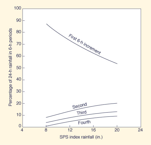
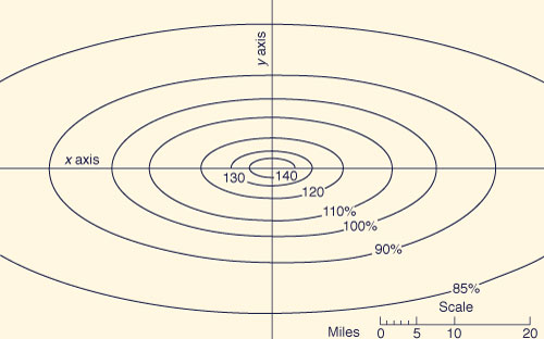
The isohyetal map shown in Fig. 14-19 is termed SPS index rainfall in order to allow conversion to storms covering areas from 10 to 20,000 mi2 and durations other than 24 h. The applicable SPS depth-area-duration chart is shown in Fig. 14-20. Criteria for the subdivision of 24-h SPS rainfall into 6-h increments is shown in Fig. 14-21. A standard 96-h SPS isohyetal pattern is shown in Fig. 14-22.
Figure 14-19 SPS index rainfall (in) [45]. |
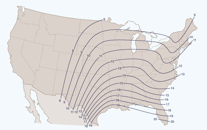
Figure 14-20 SPS depth-area-duration relation (in) [45]. |
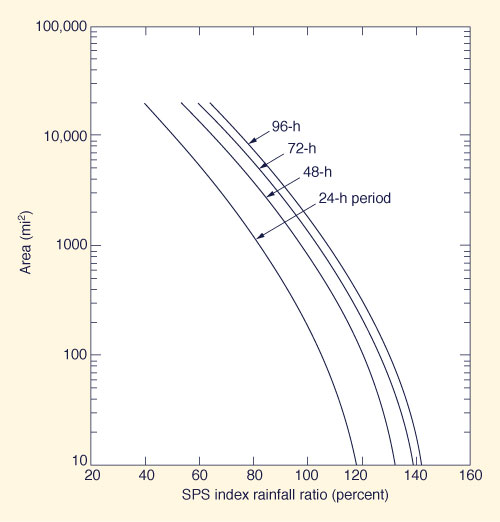
Figure 14-21 Time distribution of 24-hr SPS rainfall [45]. |
The procedure to develop an SPS estimate for small basins (less than 1000 mi2 in Corps of Engineers' practice) is the following:
Locate the drainage basin in the map of Fig. 14-19 and determine the SPS index rainfall (inches).
Enter Fig. 14-20 with the basin area to obtain the SPS index-rainfall ratios (in percent) for 24-, 48-, 72- and 96-h periods. Multiply these ratios by the SPS index rainfall obtained in step 1 and divide by 100 to calculate the 24-, 48-, 72-and 96-h SPS rainfall depths.
The 24-h SPS rainfall depth is the first of four 24-h increments in a 96-h period. Calculate the three remaining 24-h increments by subtracting the 24-, 48-, 72- and 96-h SPS values. For instance, the second 24-h increment is equal to the 48-h depth minus the 24-h depth, and so on.
Based on an appraisal of hydrologic conditions within the basin, arrange the four 24-h SPS increments in a sequence that is favorable to the production of critical runoff at project locations.
Subdivide each 24-h SPS increment into four 6-h increments in accordance with the criteria of Fig. 14-21. The same sequence of 6-h increments is assumed for each day of the SPS.
Subtract estimates of hydrologic abstractions from the 6-h incremental SPS values obtained in step 5 to calculate the effective storm hyetograph to be used in the computation of the SPF.
Figure 14-22 Standard 96-hr SPS isoyhetal pattern [45]. |
SPS Estimates for Large Basins. The basic principles involved in the preparation of SPS and SPF estimates for large drainage basins (i.e., those in excess of 1000 mi2, considered as large basins in Corps of Engineers' practice) are the same as those applicable to small basins. However, generalization of criteria becomes more difficult as the basin size increases. SPF estimates for small basins are usually governed by the maximum 6-h or 12-h rainfall associated with severe thunderstorms. For large basins, SPF estimates are generally the result of a succession of distinct rainfall events. Although the intensity and quantity of rainfall are important factors in the production of floods in a large basin, the location of successive increments of rainfall and the synchronization of intense bursts of rainfall with the progression of runoff are of equal or greater importance. Accordingly, an SPS estimate for a large basin must be based on a review of relevant meteorological data and an assessment of the hydrologic response characteristics of the basin, including the study of major floods and related historical accounts.
-------
[Under construction 210119]
14.3 NATURAL RESOURCES CONSERVATION SERVICE
|
|
All
14.4 BUREAU OF RECLAMATION
|
|
The
14.5 GEOLOGICAL SURVEY
|
|
The
QUESTIONS
|
|
PROBLEMS
|
|
REFERENCES
|
|
Hershfield, D. M. (1961). "Estimating the Probable Maximum Precipitation." Journal of the Hydraulics Division, ASCE, Vol. 87, No. HY5, September, 99-116.
Hershfield, D. M. (1965). "Method for Estimating Probable Maximum Precipitation." Journal of the American Waterworks Association, Vol. 57, No. 8, August, 965-972.
NOAA Hydrometeorological Report No. 49. (1984). "Probable Maximum Precipitation Estimates, Colorado River and Great Basin Drainages." Silver Spring, Maryland, 176 p.
NOAA Hydrometeorological Report No. 51. (1978). "Probable Maximum Precipitation Estimates, United States East of the 105th Meridian." Washington, DC, June, 100 p.
NOAA Hydrometeorological Report No. 52. (1982). "Application of Probable Maximum Precipitation Estimates - United States East of the 105th Meridian." Washington, DC, August, 182 p.
NOAA Hydrometeorological Report No. 53. (1980). "Seasonal Variation of 10-mi2 Probable Maximum Precipitation Estimates, United States East of the 105th Meridian." Silver Spring, Maryland, April, 96 p.
NOAA Hydrometeorological Report No. 55A. (1988). "Probable Maximum Precipitation Estimates, United States Between the Continental Divide an the 103rd Meridian." Silver Spring, Maryland, June, 280 p.
NOAA Hydrometeorological Report No. 57. (1994). "Probable Maximum Precipitation - Pacific Northwest States, Columbia River (including portions of Canada), Snake River, and Pacific Coastal Drainages." Silver Spring, Maryland, October, 353 p.
NOAA Hydrometeorological Report No. 58. (1998). "Probable Maximum Precipitation for California - Computational Procedures." Silver Spring, Maryland, October, 106 p.
NOAA Hydrometeorological Report No. 59. (1999). "Probable Maximum Precipitation for California." Silver Spring, Maryland, February, 419 p.
| http://engineeringhydrology.sdsu.edu |
|
160624 07:30 |