WHEN IS THE DIFFUSION WAVE APPLICABLE?
Professor Emeritus of Civil and Environmental Engineering
San Diego State University, San Diego,
California
1. INTRODUCTION
The diffusion wave is a type of wave used in flood routing.
Other types of waves are the kinematic wave and the mixed
kinematic-diffusion wave, hereafter called "mixed wave"
(Lighthill and Whitham, 1955;
Ponce and Simons, 1977).
Note that the mixed wave has been widely referred
to in the literature as "dynamic wave",
although this usage appears to be ill-advised, because it leads to a semantic
confusion with the
long-established dynamic wave of Lagrange (1788), a concept quite different from the mixed wave.
A comprehensive classification of shallow-water waves
in open-channel flow was accomplished by Ponce and Simons (1977),
who used linear stability theory to derive the celerity and attenuation functions
of all four types of shallow-water waves: (1) kinematic waves,
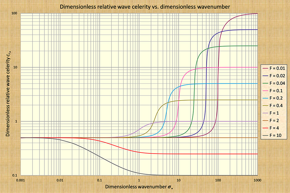
In Figure 1, kinematic waves lie along the first log cycle (to the left), while dynamic waves lie along the fifth and sixth cycles (to the right), depending on the Froude number. Mixed waves lie mostly along the fourth and fifth cycles, while diffusion waves lie along the second and third cycles.
Hydrodynamic theory asserts that if the wave celerity is a constant along the
dimensionless wavenumber, wave attenuation is zero. In Figure 1,
this condition corresponds to both kinematic waves (left of scale)
and dynamic waves (right of scale).
Conversely, if the wave celerity varies along the dimensionless wavenumber,
as in the case of a mixed wave,
wave attenuation is nonzero.
Thus, the question remains: If the kinematic
waves have no attenuation, and the mixed waves are subject to very strong
attenuation, what happens to the diffusion waves, which ostensibly lie in between them?
In this article, we make the case for the diffusion wave. We note that if the flood wave has a small amount of attenuation, the diffusion wave model will account for it, while the kinematic wave model will not. Furthermore, we show that due to the large amounts of attenuation which are predicted for mixed waves, the latter are not very likely to occur in the real world. In Section 2, we explain the nature of flood waves and make a point of the need to focus on the diffusion wave. With the applicability question clearly answered in Section 4, the time has come to hail the diffusion wave as the method of choice in flood routing engineering practice.
2. NATURE OF A FLOOD WAVE
What is the nature of a flood wave? Essentially, a flood wave is a "long" wave,
i.e., one of small dimensionless wavenumber (Fig. 1), traveling
at, or very close to, the kinematic wave celerity, and experiencing little attenuation.
Seddon (1900) pioneered
the study of flood waves, concluding
that its celerity could be expressed as
the slope of the discharge-area rating Q = αAβ,
in which Q = discharge, A = flow area, and α and β are coefficient
and exponent, respectively.
According to Seddon, the celerity of a flood wave is: c =
dQ/dA, in which dA = (1/T)dy,
with
As long as diffusion needs to be accounted for, diffusion waves may not be modeled
with kinematic waves, because the latter feature zero diffusion.
We note that in the 1980s,
kinematic waves were solved using numerical models, and the latter did feature some diffusion.
This diffusion, however, was uncontrolled numerical diffusion, and not related to the true
physical diffusion of the flood wave; therefore,
the results of the routing varied with the choice of grid size.
Could the flood wave be construed as a mixed wave,
a wave that sits on the middle-to-right of the dimensionless
wavenumber spectrum (Fig. 1)? The answer is: Not likely for typical flood waves, which hold their
stage and do not attenuate very much. If the flood wave were to attenuate strongly, it would cease to be
a flood wave, instead joining the mass of the underlying equilibrium, steady flow. Thus, we conclude that
mixed waves are not an appropriate model of flood waves, at least, not in the general case.
In the following section,
calculations of diffusion waves will confirm these statements.
Having placed aside: (a) the kinematic waves, because they lack diffusion entirely, and (b)
the mixed waves,
because they have too much diffusion, we are left only with the diffusion wave, which lies
in between kinematic and mixed waves in the dimensionless wavenumber spectrum. This is the wave
that truly embodies the nature of flood waves:
A kinematic wave featuring a small,
but perceptible, amount of
diffusion.
3. THE DIFFUSION WAVE
According to theory, the dimensionless relative celerity of a diffusion wave resembles that of a kinematic wave,
but unlike the latter, it increases, ever so slightly with the dimensionless wavenumber σ*
The discharge decreases for a negative value of
δ, causing wave attenuation,
corresponding to Froude number F < 2 (Vedernikov number V < 1);
it increases for a positive value, a logarithmic increment,
causing wave amplification, corresponding to
Froude number
Ponce and Simons (1977)
have used linear stability theory to calculate the logarithmic
decrement of the diffusion wave. The expression is:
δd = (2 π /3) σ*.
Note that in this expression, as σ* → 0, the logarithmic decrement δd → 0,
confirming that a kinematic wave is not subject to attenuation.
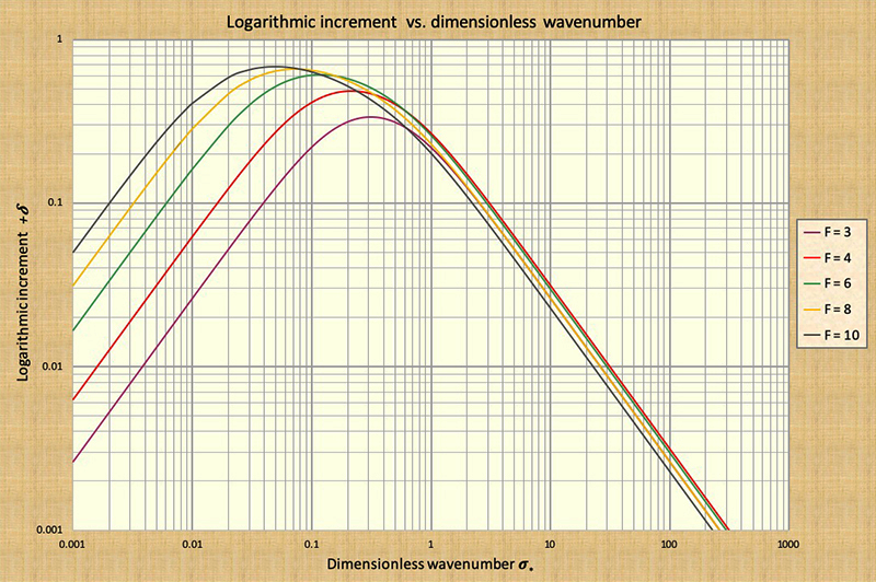
Figure 2 shows the variation of the logarithmic decrement for all wave types,
through the range of dimensionless wavenumbers
from 0.001 to 1000, for Froude numbers
Table 1 shows values of the diffusion wave logarithmic decrement δd relevant in the present context. The examination of this table leads to the conclusions summarized in Box A.
We confirm
that kinematic waves are not subject to attenuation. We also confirm that for
the midrange value of dimensionless wavenumber
σ*
> 0.17, the wave attenuation is greater than 30%, a threshold which is widely considered to be
the division
between diffusion waves (of limited wave diffusion, less than 30%)
and mixed waves (of unlimited wave diffusion, which could readily reach 100%)
We confirm the following observations, based on detailed calculations,
in reference to Fig. 1:
4. APPLICABILITY OF DIFFUSION WAVES
Having shown that diffusion waves are applicable to the flood routing
problem, we now show just how applicable they are.
Here we elaborate on the work of
Ponce and others (1978), who
established the criterion for the applicability of kinematic and diffusion waves
in terms of flood wave properties.
For the kinematic wave model, Ponce and others stated
that to achieve at least 95% accuracy of the kinematic wave solution after one period of propagation,
the dimensionless period has to satisfy the following inequality:
For the diffusion wave model, Ponce and others
compared the logarithmic decrement of the diffusion wave
δd with that of the full solution (Fig. 2), and concluded that to
achieve at least 95% accuracy of the diffusion wave solution after one period of propagation,
the dimensionless period has to satisfy the following inequality:
τ* ≥ 30.
In this case, the dimensionless period is defined as follows:
5. APPLICATION TO FIELD DATA
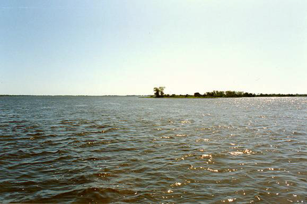
The concepts elaborated in the previous section are applied here to
the Upper Paraguay river, in Mato Grosso do Sul, Brazil,
and neighboring Bolivia.
This river features a unique geographical setting,
flowing through a continental delta
encompassing the Pantanal of Mato Grosso,
the largest wetland in the world, spanning 136,700 km2.
The geomorphological and hydrological
setting of the Upper Paraguay river has been described by
Ponce (1995).
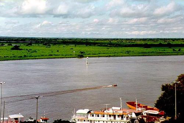
The flood hydrograph of the Upper Paraguay river, in its lower reaches, from Ladario to Porto Murtinho, comprising a distance of
Downstream of Ladario, the river stage rises from March to August,
receding from September to February. The peak stage occurs typically in the month of June
and the low stages in December.
6. CONCLUDING REMARKS
A review of diffusion waves and their use for routing flood waves has been accomplished.
Diffusion waves travel with the Seddon celerity, i.e., the kinematic wave celerity,
and are subject to little attenuation (diffusion). These properties distinctly
match those of typical flood waves. Other free-surface flow waves, namely, kinematic, mixed, and dynamic,
are either nondiffusive (kinematic and dynamic), or too diffusive (mixed).
In particular, the mixed waves are confirmed to be so greatly diffusive as to question
their mere existence altogether. Criteria for the applicability of both kinematic and diffusion waves
show that the latter, the diffusion waves, have a broader range of applicability than do the kinematic waves.
Therefore, the diffusion wave is recommended for practical applications in flood hydrology.
An application to field data from the Upper Paraguay river, in Mato Grosso do Sul, Brazil, further confirms
the findings of this study.
REFERENCES
Lagrange, J. L. de. 1788. Mécanique Analytique, Paris, part 2, section II, article 2, 192.
Seddon, J. A. 1900.
River hydraulics. Transactions, ASCE, Vol.XLIII, 179-243, June.
Lighthill, M. J. and G. B. Whitham. 1955.
On kinematic waves. I. Flood movement in long rivers.
Proceedings,
Wylie, C. R. 1966. Advanced Engineering Mathematics, 3rd ed.,
McGraw-Hill Book Co., New York, NY.
Flood Studies Report. 1975. Vol. III: Flood Routing Studies,
Natural Environment Research Council, London, England.
Ponce, V. M. and D. B. Simons. 1977.
Shallow wave propagation in open channel flow.
Journal of the Hydraulics Division, ASCE, 103(12), 1461-1476.
Ponce, V. M., R. M. Li, and D. B. Simons. 1978.
Applicability of kinematic and diffusion models.
Journal of the Hydraulics Division, ASCE, 104(3), 353-360.
Ponce, V. M. 1991. New perspective on the Vedernikov number.
Water Resources Research, Vol. 27, No. 7, 1777-1779, July.
Ponce, V. M. 1992.
Kinematic wave modeling: Where do we go from here?
International Symposium on Hydrology of Mountainous Areas, Shimla, India, May 28-30.
Ponce, V. M. 1995.
Hydrologic and environmental impact of the Parana-Paraguay waterway on the Pantanal of Mato Grosso, Brazil.
https://ponce.sdsu.edu/hydrologic_and_environmental_impact_of_the_parana_paraguay_waterway.html
Ponce, V. M. 2023.
Kinematic and dynamic waves: The definitive statement.
Online article.
| ||||||||||||||||||||||||||||||||||||||||||||||||||||||||||||||||||||||||||||||||||||||||||||||||||||||

| 230825 13:00 PDT |