KINEMATIC AND DYNAMIC WAVES: THE DEFINITIVE STATEMENT
San Diego State University, San Diego,
California
1. INTRODUCTION
This paper contrasts kinematic and dynamic waves
in open-channel flow.
2. WAVE SCALE
The "scale" of the wave is what determines whether a wave is either kinematic or dynamic.
In this context, "scale" refers not to the absolute value of wavenumber, otherwise
defined as σ = 2π /L,
but rather to its relative value, or dimensionless wavenumber,
defined as σ*
The effect of the dimensionless wavenumber is to
substantially reduce the number of
orders of magnitude required for the analysis.
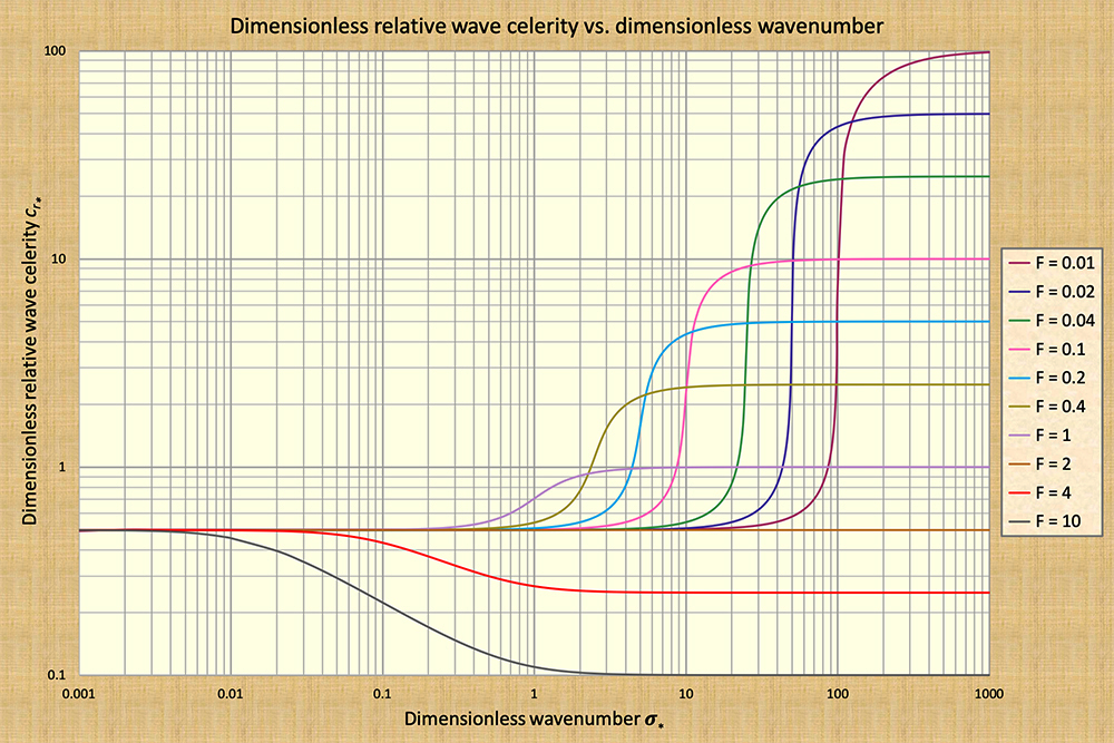
In effect, Figure 1 shows the variation of dimensionless
relative wave celerities
cr* plotted across only
six (6) orders of magnitude of
dimensionless wavenumbers
3. KINEMATIC WAVES
Figure 1 shows the plot of relative dimensionless wave celerities
across the dimensionless wavenumber spectrum, from very small, corresponding to kinematic waves
(σ* = 0.001), to
very large, corresponding to dynamic waves
Note that throughout the dimensionless wavenumber
spectrum σ*,
the dimensionless relative wave celerity
cr*
is a constant and equal to cr* = 0.5
only for Froude number F = 2. We note specifically that
this flow condition corresponds to Chezy friction in a hydraulically wide channel (se Box B below)
(Ponce and Simons, 1977). This is the physical condition
for which all wave scales travel with the same celerity, representing the onset of flow stability/instability:
stability for F < 2, and instability F > 2.
Further examination of Fig. 1 reveals that the kinematic waves are positioned to the left of the figure, in a fashion asymptotic to the constant value cr* = 0.5 in the extreme left of the figure, which corresponds to the dimensionless relative kinematic wave celerity for Chezy friction in a hydraulically wide channel (Ponce, 2014). The concept of kinematic wave celerity, which is akin to that of flood wave celerity, is due to Seddon (1900), who first derived the formula bearing his name. Related expressions are contained in the following box.
We wish to reiterate that kinematic waves do exist, admittedly only as a convenient approximation, typically on the left side of the dimensionless wavenumber spectrum. They correspond to a large class of flood waves, particularly those that are subject to very little (or otherwise, negligible) attenuation. They also may show up in overland flow modeling, wherein the prevailing bottom slopes are large enough to trigger a kinematic flow condition and the resulting kinematic waves (Woolhiser and Liggett, 1967). The early work of Seddon (1900), followed by that of Lighthill and Whitham (1955), have been important milestones in advancing kinematic wave applications in hydraulic and hydrologic engineering.
4. DYNAMIC WAVES
Dynamic waves lie to the right of the dimensionless wavenumber spectrum, and the dimensionless relative
wave celerities are constant across the dimensionless wavenumbers,
and a function of the Froude number of the equilibium flow, with smaller celerities
corresponding to larger Froude numbers, and vice versa; for instance,
cr*
Figure 1 shows the values of dimensionless relative dynamic
wave celerities cdrd lying to
the right of the figure. For instance, using the last definition of cdrd (labeled 8
in Box C above), it follows that:
We have shown that Figure 1 correctly depicts the values of dimensionless relative dynamic, or Lagrange, celerities. Thus, we show that Figure 1 encompasses both kinematic and dynamic waves in the same figure. Reiterating, dynamic waves lie to the right of the dimensionless wavenumber σ*, wherein the dimensionless relative dynamic wave celerities are a function of the Froude number of the equilibrium flow. According to Ponce and Simons (1977), the attenuation of a dynamic wave is zero, i.e., dynamic waves are not subject to attenuation (i.e., wave dissipation), at least in a one-dimensional analysis. This conclusion follows directly from Fig. 1, because in the applicable dynamic range, toward the extreme right of the figure, the wave celerity is shown to be constant and, thus, independent of scale. This conclusion confirms that a dynamic wave is not subject to attenuation. Thus, a dynamic wave is a comparatively small surface wave, featuring a correspondingly small dimensionless wavenumber, traveling at a dimensionless relative celerity which is the reciprocal of the Froude number of the equilibrium flow, and it is not subject to attenuation. Dynamic waves do exist, admittedly only as a convenient approximation, typically on the right side of the dimensionless wavenumber spectrum. They correspond to a class of relatively short surface waves, particularly those that are subject to very little or negligible attenuation.
5. MIXED KINEMATIC-DYNAMIC WAVES
Granted that kinematic waves lie to the left of the dimensionless wavenumber spectrum.
while dynamic waves lie to the right, with neither being subject to attenuation.
This is due to the constancy of the respective celerities within the specified range of analysis.
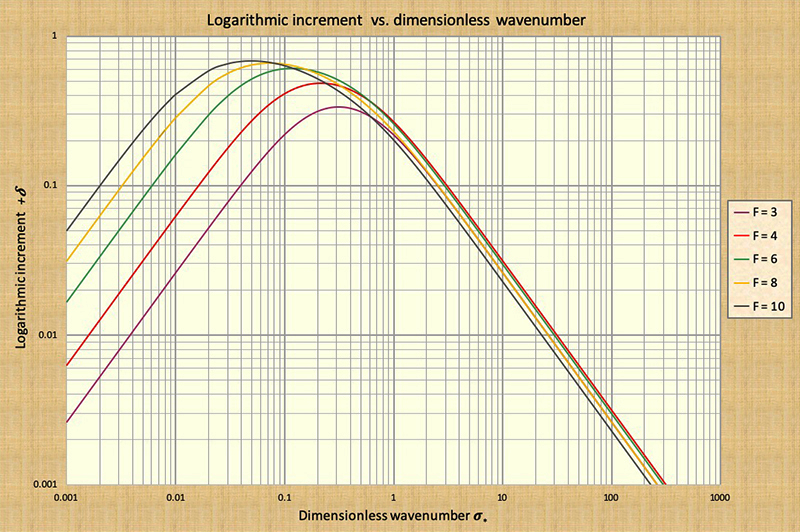
Wave attenuation is due to the varying group celerity,
which attains a maximum
value, depending on the Froude number, toward (the right of) the midrange dimensionless wavenumbers.
The greater the variability in celerity (with dimensionless wavenumber), the greater the wave attenuation, the latter
shown to increase with equilibrium flow Froude numbers; compare Figs. 1 and 2.
We conclude that toward the middle of the dimensionless wavenumber spectrum, wave attenuation is a maximum, while toward the extremes, both left and right, it is a minimum (Fig. 2). Correspondingly, similar conclusions apply for wave amplification, as observed in Fig. 3.
Therefore, mixed kinematic-dynamic waves are subject to varying attenuation,
from mild to very strong, with the amount of attenuation varying
with the value of dimensionless wavenumber, relative to the location of the
point of inflection in the celerity-wave number curve. In certain cases, the mixed kinematic-dynamic wave
may be so strongly dissipative as to defy calculation altogether.
In closing, we wish to point out that our "mixed kinematic-dynamic waves" have been, for the
past nearly 50 years, simply referred to as "dynamic waves",
thereby contributing to the semantic confusion
6. DIFFUSION WAVES
Having established conclusively that neither kinematic nor dynamic waves attenuate,
and conversely, that mixed kinematic-dynamic
waves could be subject to very strong attenuation, we feature here another type of intermediate
wave, which, as far as the value of dimensionless wavenumber,
lies in between kinematic and mixed kinematic-dynamic waves.
This wave is properly a kinematic wave with diffusion,
to follow Lighthill and Whitham (1955),
or, more concisely, a diffusion wave, to follow Ponce and Simons (1977). It
is defined by including, in the wave definition, the pressure-gradient term.
We conclude that wave diffusion is produced by: (1) the interaction of the pressure-gradient term with the friction and gravity terms, as in the diffusion wave; or (2) by the interaction of all the (four) terms in the equation of motion, i.e., as in the mixed kinematic-dynamic wave.
The diffusion of the diffusion wave is described by the logarithmic decrement δ =
- 2 π (σ* / 3),
which is applicable only within the range of dimensionless wavenumbers
wherein the diffusion wave is
prevalent, i.e., within a narrow range between that of kinematic waves (extreme left of chart)
and that of mixed kinematic-dynamic waves (toward the center right of the chart)
Diffusion waves turn out to be more common than either kinematic or mixed kinematic-dynamic waves and, therefore, this helps explain their growing popularity in practical applications. Kinematic waves do not attenuate, and mixed kinematic-dynamic waves may actually attenuate too much. Diffusion waves find their demonstrably best applicability in the routing of flood waves, which typically are subjected to some, but not too much, wave attenuation.
7. SUMMARY
A review of
several relevant types of shallow-water waves in open-channel flow are discussed and compared
with regard to their celerity and attenuation properties. These waves are: (1) kinematic waves,
Kinematic waves travel with a constant celerity and are non-diffusive.
The constant celerity of kinematic waves has been referred to in the flood routing literature
as the 'Seddon celerity'.
Dynamic waves travel with a constant celerity and are non-diffusive.
The constant celerity of dynamic waves is referred to as the 'Lagrange celerity', applicable to
"short" waves in open-channel flow.
Mixed kinematic-dynamic waves travel with a celerity which varies with the dimensionless
wavenumber, and this property gives them the capability to diffuse, i.e., to attenuate or dissipate.
Diffusion waves lie in between kinematic and mixed kinematic-dynamic waves, in terms of relative scale.
These waves travel approximately with the Seddon celerity and are shown to be
mildly diffusive; therefore, they remain
admirably suited to the modeling of flood waves.
REFERENCES
Fread, D. L. 1985. "Channel Routing," in Hydrological Forecasting,
M. G. Anderson and T. P. Burt, eds. New York: John Wiley.
Ponce, V. M. and D. B. Simons. 1977.
Shallow wave propagation in open channel flow.
Journal of Hydraulic Engineering, ASCE, 103(12), 1461-1476.
Ponce, V. M. 1991.
New perspective on the Vedernikov number.
Water Resources Research, Vol. 27, No. 7, 1777-1779, July.
Ponce, V. M. 2014.
Fundamentals of Open-channel Hydraulics.
Online text.
Seddon, J. A. 1900. River hydraulics. Transactions, ASCE, Vol. XLIII, 179-243, June.
Woolhiser, D. A. and J. A. Liggett. 1967.
Unsteady one-dimensional flow over a plane: The rising hydrograph.
|

| 230816 06:30 PDT |