Sediment transport

CIVE 530 - OPEN-CHANNEL HYDRAULICS
LECTURE 17B: SEDIMENTATION ENGINEERING II

17.3 SEDIMENT TRANSPORT

Sediment transport refers to the entrainment and movement of sediments by flowing water.
An understanding of the principles of sediment transport is essential for the interpretation and solution of many hydraulic, hydrologic, and water resources engineering problems.
The study of sediment transport can be divided into:

sediment transport mechanics,
sediment transport prediction, and
sediment routing.

Sediment transport mechanics refers to the fundamental processes by which sediment is entrained and transported by flowing water.
Sediment transport prediction refers to the methods and techniques to predict the equilibrium or steady rate of sediment transport in streams and rivers.
The prediction of sediment transport is accomplished by a sediment transport formula.
Sediment routing refers to the nonequilibrium or unsteady sediment transport processes, the net result of which is either the aggradation or degradation of streams or river beds.
The energy and turbulence of the flow gives streams and rivers the capacity to entrain and transport sediment.
Entrainment and transport is a function of the vertical velocity gradient near the streambed.
The sediment being transported can originate in either upland or channel sources.
A significant feature of sediment transport is the entrainment and transport by the flow of the material constituting the streambed.
Thus, sediment transport is the mechanism by which streams and rivers determine their own cross sectional shapes and boundary roughness.

SEDIMENT TRANSPORT MECHANICS

Sediment load or sediment discharge is the total amount of sediment transported by a stream or river past a given point, expressed in terms of weight per unit volume.
Based on the predominant mode of transport, sediment load can be classified into:
bed load, and
suspended load.

Bed load is the fraction of sediment load that moves by saltation and rolling along the streambed, primarily by action of bottom shear stresses caused by vertical velocity gradients.
Suspended load is the fraction of sediment load that moves in suspension by the action of turbulence.
Particles transported as bed load are coarser than particles transported as suspended load.
Some particles may move as bed load at one point, and as suspended load at another.
Based on whether the particle sizes are represented in the streambed, sediment load can be classified into:
bed material load, and
fine material load.

Bed material load is the fraction of sediment load whose particle sizes are significantly represented in the streambed.
Fine material load, commonly referred to as "wash load," is the fraction of sediment load whose particle sizes are not significantly represented in the streambed.
Bed material load is the coarser fraction of sediment load, which may have originated in the channel bed, and that may be subject to deposition under certain conditions.
Wash load is the finer fraction of sediment load, that has not originated in the channel bed, and that is not likely to deposit.
Wash load is largely unaffected by the hydraulics of the flow.
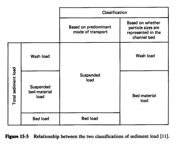
The relationship between the two classifications of sediment load is shown in Fig. 15-5.
This figure shows that the concepts of bed load and wash load are mutually exclusive.
The middle overlap is the suspended bed material load, i.e., the fraction of sediment load that moves in suspended mode and is composed of particle sizes that are represented in the channel bed.

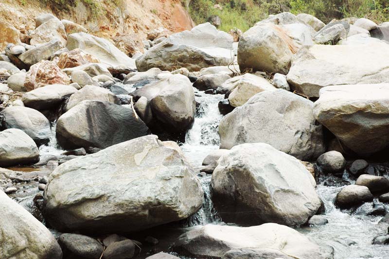
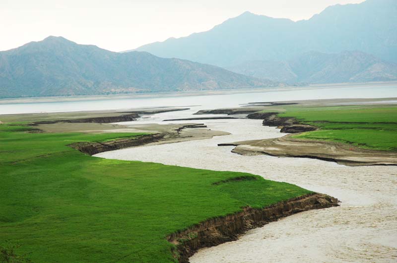
Rachichuela wash, in La Leche basin, northern Peru.

Initiation of Motion

Water flowing over a streambed has a marked vertical velocity gradient near the streambed.
This velocity gradient exerts a shear stress on the particles lying on the streambed, i.e., a bottom shear stress.
For wide channels, the bottom shear stress can be approximated by the following formula:

τ_o = γ d S
in which:
τ_o = bottom shear stress;
γ = specific weight of water;
d = flow depth; and
S = equilibrium or energy slope.

There is a threshold value of bottom shear stress above which the particles actually begin to move.
This threshold value is referred to as the critical bottom shear stress, or critical stractive stress.
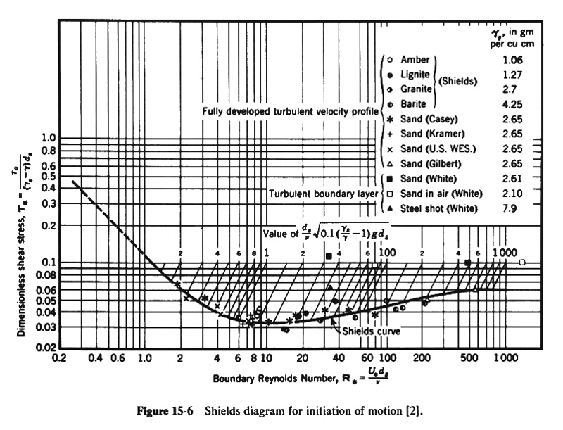
The Shields curve, shown in Fig. 5-6, represent the earliest attempt to combine theoretical and empirical approaches to estimate critical tractive stress.
The Shields curve depicts the threshold of motion, i.e., the condition separating motion (above the curve) from no motion (below the curve).

The abscissa in the Shields diagram is the boundary Reynolds number, defined as:

R_* = U_*d_s/ν

in which:
R_* = boundary Reynolds number;
U_* = shear velocity;
d_s = mean particle diameter; and
ν = kinematic viscosity of the water.
The shear velocity is defined as:

U_* = (τ_o/ρ)^1/2

in which ρ = density of water.
The ordinate in the Shields diagram is the dimensionless tractive stress, defined as:

τ_* = τ_o/[(γ_s - γ) d_s]

in which τ_o = dimensionless tractive stress.
The Shields diagram indicates that, within a midrage of boundary Reynolds numbers (approximately 2-200), the dimensionless critical tractive stress can be taken as a constant for practical purposes.
Within this range, the critical tractive stress is proportional to the sediment particle size.
For instance, assuming τ_* = 0.04 from the Shields diagram:

τ_c = 0.04 (γ_s - γ) d_s]

in which &tau_c = = critical tractive stress.
For quartz particles, for which γ_s = 2.65 * 62.4 lb/ft³:

τ_c = 0.34 d_s

in which τ_c is in lbs/ft² and d_s in inches.
Extensive experimental studies by Lane have shown that the coefficient in the above equation is around 0.5.
However, Lane used the d₇₅ (diameter for which 75% by weight is finer) instead of the d₅₀ used by Shields.

Example 15-5.
Based on the Shields criterion, determine whether a 3-mm quartz particle is at rest or moving under a 7-ft flow depth with channel slope S_o = 0.0001. Asssume T = 70^oF.
Solution:
The bottom shear stress is:
&tau_o = γ d S = 62.4 × 7.0 × 0.0001 = 0.0437 lb/ft²
The dimensionless tractive stress is:
τ_* = &tau_o/[(γ_s - γ) d_s] = 0.0437/[(2.65 - 1.00) × 62.4 × 3.0/(25.4 × 12)] = 0.0431.
The shear velocity is:
U_* = (&tau_o/ρ)^1/2 = (0.0437/1.94)^1/2 = 0.150 ft/s.
The kinematic viscosity is:
ν = 1.058 × 10^-5 ft²/s.
The boundary Reynolds number is:
R_* = U_*d_s/ν = 0.150 × [3.0/(25.4 × 12)] /(1.058 × 10^-5) = 140.
For R_* = 140, the dimensionless critical tractive stress is: τ_*c = 0.048.
Since τ_* = 0.0431 < τ_*c = 0.048
Thus, the particle is at rest.

Example 15-5 Online.
Solve this example using online shields.
Boundary Reynolds number R_* = 139.6
Dimensionless tractive stress τ_* = 0.0431
Dimensionless critical tractive stress τ_*c = 0.0482
τ_* = 0.0431 < τ_*c = 0.0482
Thus, the particle is at rest.
Forms of bed roughness

Streams and rivers create their own geometry.
Alluvial rivers determine their cross-sectional shape and boundary friction as a function of the prevailing water and sediment discharge.
An inherent property of river flows is their tendency to minimize changes in stage caused by changes in discharge.
This is accomplished through a continuous adjustment in boundary friction in such a way that high values of friction prevail during low flows and low values prevail during high flows.
Adjustments in boundary friction are made possible by the existence of bedforms, which develop during low flows only to be obliterated during high flows.
Boundary friction consists of two parts:
grain roughness, and
form roughness.

Grain roughness is a function of particle size.
Form roughness is a function of the size and extent of bedforms.
Grain roughness is essentially a constant, while form roughness varies with the flow.

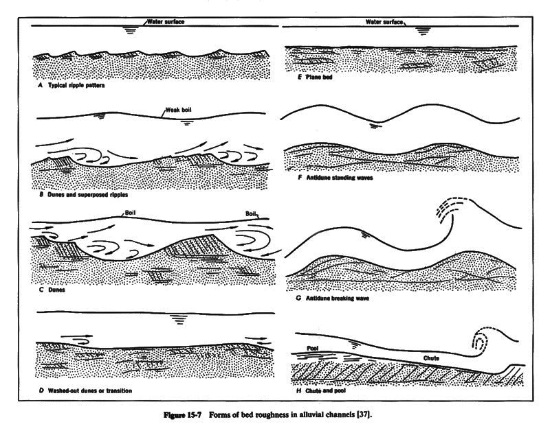
Several forms of bed roughness can exist in rivers.
In the absence of sediment movement, the bed configuration is that of plane bed with no sediment motion.
With sediment movement, the following forms of bed roughness have been identified:
ripples,
dunes and superimposed ripples,
dunes,
washed-out dunes, or transition [to upper regime],
plane bed with sediment motion,
antidunes, and
chutes and pools.

Sketches of these bed configurations are shown in Fig. 15-7.

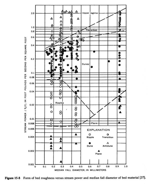
The occurrence of different forms of bed roughness is related to the median fall diameter of the bed particles and the stream power of the flow.
Stream power is defined as the product of bottom shear stress and mean velocity.

SP = τ_o V

The bedform-stream power-median fall diameter relation is shown in Fig. 15-8.

For low stream power, there is no bedload transport.
This is the condition of plane bed with no sediment motion.
An increase in stream power leads to ripples, then to dunes with superimposed ripples, and subsequently dunes.
Ripples are a rare occurrence for sediments coarser than 0.6 mm.
Dunes occur and flow velocities and sediment loads that are greater than ripples.
Plane bed with sediment motion occurs when the stream power is large enough to obliterate the dunes, essentially eliminating form roughness.
The plane bed represents the condition of minimum boundary friction.
For high values of stream power, antidunes form in conjunction with surface waves, usually under supercritical flow conditions.
In very steep streams, the bed configuration resembles a series of chutes and pools.

The assessment of bedform type has practical implications.
Bedforms determine boundary roughness; in turn, boundary roughness determines river stages.
Ripples are associate with values of Manning n in the range 0.018-0.030, with form roughness usually a fraction of grain roughness.
Dunes are associated with values of Manning n in the range 0.020-0.040, with form roughness of the same order as grain roughness.
Plane bed with sediment motion is associated with relatively low n values, in the range 0.012-0.015, with minimal form roughness.
Concentration of suspended sediment

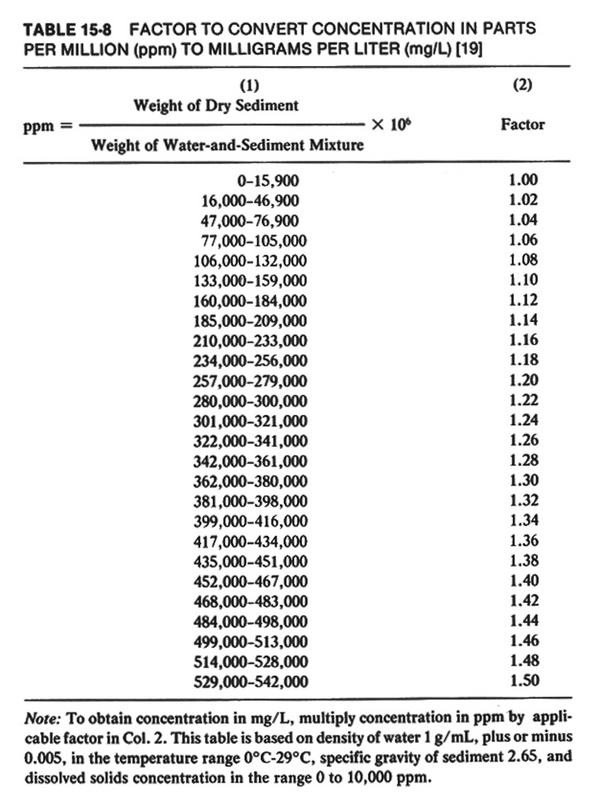
For a given volume of water-sediment mixture, the suspended sediment concentration is the ratio of the weight of dry sediment to the weight of the water-sediment mixture, expressed in parts per million (ppm).
To convert the concentration in ppm to concentration in mg/L, the applicable factor ranges from 1 for concentrations between 0 and 15,900 ppm, and 1.5 for concentrations in the range 529,000-542,000 (see Table 15-8).

The suspended sediment concentration varies within the vertical flow depth.
It is high near the streambed and lower near the water surface.
The coarsest sediment fractions exhibit the greatest variation in concentration with flow depth.
The finer fractions, silt and clay, show a tendency for a nearly uniform distribution of suspended sediment concentration with flow depth.

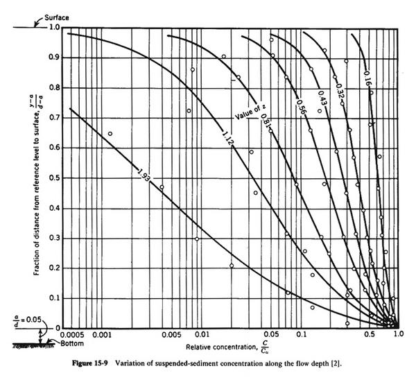
Fig. 15-9 shows the variation of suspended sediment concentration along the flow depth.

In this figure, y is the fraction of flow depth d meaasured from the channel bottom, and a is the reference distance measured from the channel bottom.
The abscissa shows C/C_a, where C_a is the sediment concentration at the reference distance and C is the sediment concentration at a distance (y - a).
The ordinates show the dimensionless ratio (y - a) / (d - a).
The curve parameter is the Rouse number:

z = w /(βκU_*)

in which:
z = Rouse number (dimensionless);
w = fall velocity of sediment particles;
β = a coefficient relating mass and momentum transfer (β ≅ 1 for fine sediments);
κ = von Karman's constant (κ = 0.4 for clear fluids); and
U_* = shear velocity.
For high Rouse numbers, the variation of suspended sediment concentration along the flow depth is quite marked.
For low Rouse numbers, there is a tendency for greater uniformity of suspended sediment concentration along the flow depth.

SEDIMENT TRANSPORT PREDICTION

Sediment load, sediment discharge, and sediment transport rate are synonymous.
Bed load, suspended bed material load, and wash load are mutually exclusive.
Sediment transport prediction refers to the estimation of sediment transport rates under equilibrium flow conditions.
There are many formulas for the prediction of sediment transport.
Most formulas compute only bed material load, consisting of bed load and suspended bed material load.
A few compute total sediment load, which consists of bed load, suspended bed material load, and wash load.
Some compute bed load and suspended bed material load separately.
Sediment transport formulas have empirical components; therefore, they have a range of applicability.
Duboys formula

The Duboys formula is widely recognized as one of the earliest attempts to develop a sediment transport predictor.
The Duboys formula is:

q_s = ψ_D τ_o(τ_o - τ_c)

in which
q_s = bed material transport rate per unit of channel width, in lbs/sec/ft;
ψ_D = parameter function of particle size, in ft³/lb/sec;
τ_o = bottom shear stress in lb/ft²; and
τ_c = critical shear stress in lb/ft².
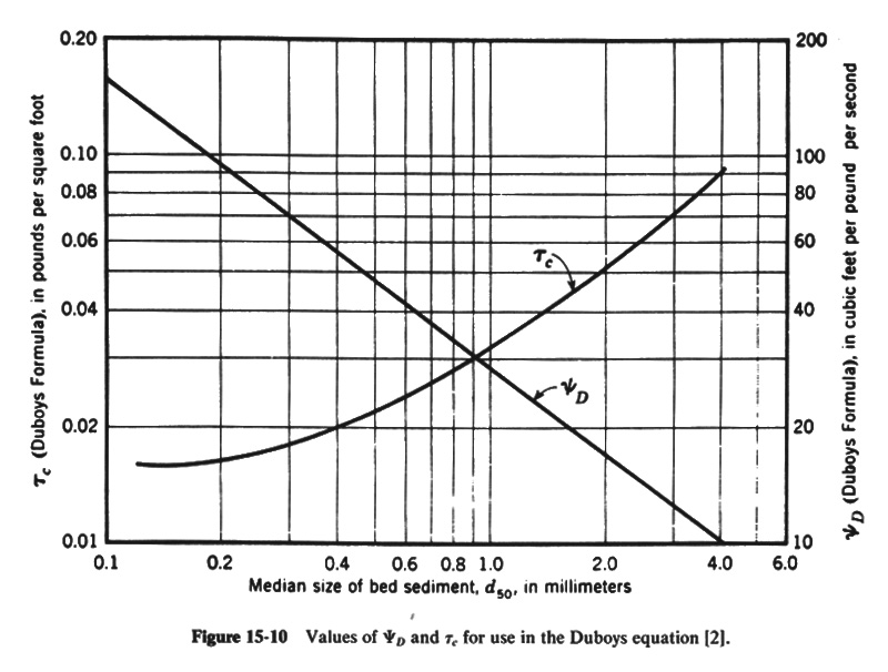
Values of ψ_D and τ_c are given in Fig. 15-10.

Example 15-6.
Given d = 12 ft, b = 320 ft, S_o = 0.0001, and d₅₀ = 0.6 mm. Calculate the bed material transport rate by the Duboys formula.
Solution:
The bottom shear stress is:
τ_o = γ d S = 62.4 × 12.0 × 0.0001 = 0.07488 lb/ft²
From Fig. 15-10: ψ_D = 42 ft³/lb/sec.
From Fig. 15-10: τ_c = 0.0245 lb/ft².
q_s = 42 × 0.07488 × (0.07488 - 0.0245) = 0.158 lb/sec/ft.
Q_s = 0.158 × 320 = 50.56 lb/sec.

Example 15-6 Online.
Solve this example using online duboys.
Q_s = 50.55 lb/sec.
Meyer-Peter formula

The development of the Meyer-Peter formula was based on flume data, with particle sizes in the range 3-28 mm.
The formula is applicable to coarse sediment transport where form roughness is negligible.
The Meyer-Peter formula is:

q_s = (39.25 q^2/3S_o - 9.95 d₅₀ )^3/2

in which
q_s = bed material transport rate per unit of channel width, in lbs/sec/ft;
q = water discharge per unit of channel width, in ft³/sec/ft;
S_o = equilibrium channel slope; and
d₅₀ = median particle size, in ft.

Example 15-7.
Given d = 2 ft, b = 25 ft, v = 6 ft/sec, S_o = 0.008, and d₅₀ = 22 mm. Calculate the bed-material transport rate by the Meyer-Peter formula.
Solution:
q = vd = 6 × 2 = 12 ft³/sec/ft.
q_s = {(39.25 × 12^2/3 × 0.008) - [9.95 × 22/(25.4 × 12)]} = 0.894 lb/sec/ft.
Q_s = q_s b = 0.894 × 25 = 22.35 lb/sec.

Example 15-7 Online.
Solve this example using online meyer-peter.
q_s = = 0.893 lb/sec/ft.
Q_s = 22.337 lb/sec.
Einstein's bed-load function

In 1950, Einstein published a procedure for the computation of bed material transport rate by size fractions.
The method was developed based on theoretical considerations of turbulent flow, supported by laboratory and field data.
Einstein is credited with the separation of boundary friction into grain and form roughness.
Einstein is also credited with using the statistical properties of turbulence to explain the mechanics of sediment transport.
Einstein's bed-load function first computes the bed-load transport rate.
Then it uses the bed-load transport rate to aid in the integration of the product of the suspended sediment concentration profile and the flow velocity profile, to determine the suspended bed-material transport rate, by individual size fractions.

Modified Einstein Procedure

The Modified Einstein Procedure (MEP) was developed by Colby and Hembree in 1955.
The method includes actual measurements of suspended load into the framework of the original Einstein method.
Typically, measurements of suspended load do not include
the bed load, and
the fraction of suspended load moving too close to the streambed to be effectively sampled.

The Modified Einstein Procedure calculates total sediment load, measured and unmeasured, bed material and wash load, by size fractions based on measurements of suspended load and geometric and hydraulic properties.
The MEP is the most complete predictor of total sediment load to date.

Example Modified Einstein Procedure Online.
Use online modified einstein with the following data:
Discharge Q = 240 ft³/sec
Mean velocity u = 2.1 ft/s
Flow depth d = 1.1 ft
Channel width w = 110 ft
Water temperature T = 70 ^oF
Diameter D₆₅ = 0.00105 ft
Diameter D₃₅ = 0.00075 ft
Measured concentration C = 245
Vertical distance not sampled d_n = 0.3 ft
Mean depth at sampling verticals d_s = 1.2 ft
Fraction of bed material in each size range i_b (9 values): 0.,0.,0.38,0.50,0.05,0.01,0.01,0.,0.
Percentage of suspended material in each size range Q'_s (9 values): 22.,25.,42.,11.,0.,0.,0.,0.,0.
Use original 1955 procedure.

Solution:
Computed load with online modified einstein: 414.2 tons/day.

Colby 1957 method

The Colby 1957 is based on the same measurements that led to the development of the Modified Einstein Procedure.
However, the Colby 1957 method does not account for sediment transport rate by size fractions.
The Colby 1957 method provides the total bed-material discharge, i.e., the sum of measured and unmeasured loads.
The following data are needed:
mean flow depth d,
mean channel width b,
mean velocity v, and
measured concentration of suspended bed-material discharge C_m.

The procedure is as follows:
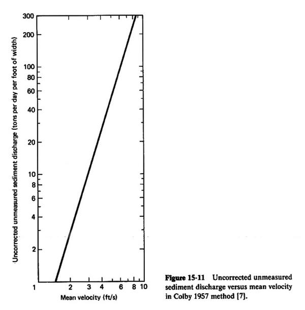
Use Fig. 15-11

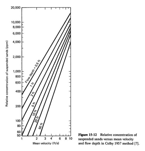
Use Fig. 15-12 to obtain the relative concentration of suspended sands C_r (in ppm) as a function of mean velocity and flow depth.

Calculate the availability ratio C_m/C_r. [Use Table 15-8 to convert C_m in ppm to mg/L].
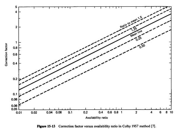
Use the mean line in Fig. 15-13 and the availability ratio to obtain the correction factor C.

Calculate the unmeasured sediment discharge q_u = C q_u'
Calculate the total sediment discharge (in tons per day per foot of width):
q_s = 0.0027 C_mq + q_u
in which C_m is in mg/L.

Example 15-8.
Given flow depth d = 10 ft, channel width b = 300 ft, mean velocity v = 3 fps, measured concentration of suspended sediment C_m = 100 ppm. Calculate the total bed-material discharge by the Colby 1957 method.
Solution:
From Fig. 15-11, the uncorrected unmeasured sediment discharge is: q_u' = 10 tons/day/ft
From Fig. 15-12, the relative concentration of suspended sands is: C_r = 380 ppm.
The availability ratio is: C_m/C_r = 100/380 = 0.26.
From Fig. 15-13, the correction factor is: C = 0.6
q_u = 0.6 × 10 = 6 tons/day/ft
q = vd = 3 × 10 = 30 cfs/ft.
q_s = 0.0027 C_mq + q_u = (0.0027 × 100 × 30) + 6 = 14.1 tons/day/ft.
Q_s = 14.1 × 300 = 4230 tons/day

Example 15-8 Online.
Solve this example using online colby 1957.
q_s = 14.104 tons/day/ft
Q_s = 4231.15 tons/day

Colby 1964 method

In 1964, Colby published a method to calculate discharge of sands in sand-bed streams and rivers.
The development of the method was guided by the Einstein bed-load function and supported by large amounts of laboratory and field data.
The method provides a good prediction of transport rates in the sand-size particles.
The following data are needed:
mean flow depth d,
mean channel width b,
mean velocity v,
water temperature,
concentration of fine-material load (wash load), and
median bed-material size.

The procedure is as follows:

Use Fig. 15-14 to determine the uncorrected discharge of sands q_u (in tons/day/ft) as a function of mean velocity, flow depth, and sediment size.

For water temperature of 60^oF, wash load less than 1000 ppm, and sediment size in the range 0.2-0.3, no further calculations are required, and q_u is the discharge of sands q_s.
For conditions other than the preceding, use Fig. 15-15 to obtain the correction factor:
k₁ as a function of flow depth and water temperature,
k₂ as a function of flow depth and concentration of fine-material load, and
k₃ as a function of median size of bed material.

The discharge of sands is given by the following formula:
q_s = [ 1 + (k₁k₂ - 1) k₃ ] q_u

Example 15-9.
Given flow depth d = 1 ft, channel width b = 30 ft, mean velocity v = 2 fps, water temperature 50^oF, wash load concentration C_w = 10,000 ppm, and median bed-material size d₅₀ = 0.1 mm. Calculate the total bed-material discharge by the Colby 1964 method.
Solution:
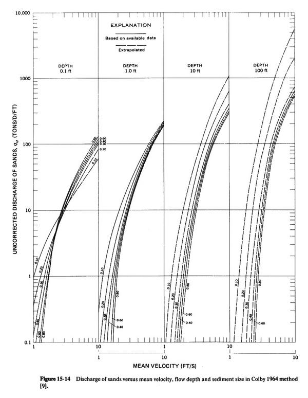
From Fig. 15-14: q_u = 9.0 tons/day/ft
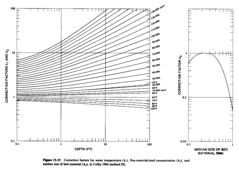
From Fig. 15-15: k₁ = 1.14, k₂ = 1.22, and k₃ = 0.6.
q_s = [ 1 + (k₁k₂ - 1) k₃ ] q_u = [ 1 + (1.14 × 1.22 - 1) × 0.6 ] × 9.0 = 11.11 tons/day/ft.
Q_s = 11.11 × 30 = 333.3 tons/day.

Example 15-9 Online.
Solve this example using online colby.
q_s = 11.11 tons/day/ft
Q_s = 333.31 tons/day

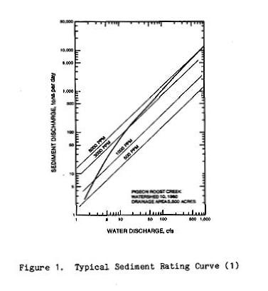
SEDIMENT RATING CURVES

A sediment rating curve is the relationship between sediment discharge and water discharge at a given gaging station.
The rating assumes steady equilibrium flow conditions.
The curve shows water discharge in the abscissas and sediment discharge in the ordinates.
This plot is obtained by simultaneous measurements of water and sediment discharge, or by the use of sediment transport formulas.
For low water discharges, the sediment rating curve usually plots as a straight line on logarithmic paper, showing an increase in sediment concentration with water discharge.
For high discharges, the sediment rating curve has a tendency to curve slightly downward, approaching a line of equal sediment concentration.

Like the single-valued stage-discharge rating, the single-valued sediment rating curve is strictly valid only for steady equilibrium flow conditions.
For strongly unsteady flows, the existence of loops in both water and sediment rating curves has been demonstrated.
These loops are complex in nature, and are likely to vary from flood to flood.
In practice, loops in water and sediment discharge are commonly disregarded.
The sediment rating curve.

SEDIMENT ROUTING

The calculation of sediment yield is lumped, i.e., it does not provide a measure of spatial or temporal variability of sediment production within the catchment.
Sediment transport formulas are based on the assumption of steady uniform flow.
Sediment routing refers to the distributed and unsteady calculation of sediment production, transport, and deposition in catchments, streams, rivers, reservoirs, and estuaries.
Sediment routing is ideally suited to the computer.
Sediment routing is used where the description of spatial and temporal variations of sediment production, transport, and deposition is warranted.
Sediment routing is used for the analysis of aggradation and degradation in streams and rivers.
The 2007 version of HEC-RAS has sediment routing, extending the HEC-6 model.

THE LANE RELATION

In 1955, Lane presented a relation to explain aggradation and degradation in alluvial channels and rivers.
It states the proportionality of water and sediment discharge.
The Lane relation is:

Q_sd ∝ Q_wS

in which:
Q_s = sediment discharge;
d = particle diameter (size of sediment);
Q_w = water discharge; and
S = slope of the stream.
Since the sediment concentration C = Q_s / Q_w, it follows that the Lane relation states that the sediment concentration is directly proportional to the slope and inversely proportional to the sediment size.
According to Lane, the change in one of these quantities will trigger adjustments in the other quantities.
For instance, if sediment discharge Q_s is decreased, the slope will decrease accordingly, causing degradation.
If sediment discharge Q_s is increased, the slope will increase, causing aggradation.
If the water discharge Q_w is increased, the slope will decrease, causing degradation.
The Modified Lane relation states the original Lane relation in dimensionless form:

Q_s(d/R)^1/3 ∝ Q_wS

in which R = hydraulic radius.
The ratio d/R is the relative roughness.
Unlike the original Lane relation, this new relation is dimensionless.

17.4 SEDIMENT DEPOSITION IN RESERVOIRS

The concepts of sediment yield and sediment transport are essential to the study of sediment deposition in reservoirs.
Sediment is transported downstream by the action of flowing water.
As the water is detained in an instream reservoir, deposition of sediment takes place.
Sediment deposition occurs in the vicinity of reservoirs, as shown in Fig. 15-16.

Deposition of the coarser fractions takes place near the entrance to the reservoir.
The delta continues to grow in the direction of the dam, until it eventually fills up the entire reservoir volume.
The process is quite slow but relentless.
Typically reservoirs may take 50 to 100 years to fill, and in some instances, up to 500 years or more.

Sediment deposition at mouth of inlet to Tinajones reservoir, Chiclayo, Peru.

The rate of sediment deposition in reservoirs is a matter or considerable economic and practical interest.
It has been said that all reservoirs will fill up with sediment eventually.
In an extreme case, the filling can occur in one event, as with the sediment retention basins.

RESERVOIR TRAP EFFICIENCY

The difference between incoming and outgoing sediment is the sediment deposited in the reservoir.
The incoming sediment is quantified by the sediment yield.
The outgoing sediment is quantified by the trap efficiency.
Trap efficiency refers to the ability of the reservoir to entrap (settle) sediments.
Trap efficiency is the ratio of trapped sediments to incoming sediments, in percentage.
Trap efficiency is a function of:
the ratio of reservoir volume to mean annual runoff volume, and
The sediment characteristics.

The following procedure is use to determine trap efficiency:

Determine the reservoir capacity C (hm³ or ac-ft).
Determine the mean annual runoff volume inflow I to the reservoi (hm³ or ac-ft).
Use Fig. 15-17 to determine the percentage trap efficiency as a function of the ratio C/I for any one of three sediment characteristics (based on texture type).

Fig. 15-17 The Brune curves for reservoir trap efficiency.

RESERVOIR DESIGN LIFE

The design life of a reservoir is the period required to fulfill its intended purpose.
Structures designed by the NRCS have a design life of 50 to 100 years.
Due to reservoir sedimentation, provisions are made to guarantee the full design reservoir water-storage capacity for the planned design life.
This may entail:
cleaning out sediment deposits at predetermined intervals during the life of the structure, or
providing a reservoir storage capacity large enough to store all the accumulated sediment deposits without encroachment on the designed water-storage volume.

Calculations of sediment-filling rates are part of the design of reservoir projects.

DISTRIBUTION OF SEDIMENT DEPOSITS

The distribution of sediment deposits may be such as to materiall affect the operation of the reservoir.
The amount and types of sediment deposits vary with the sediment itself, the nature of the approach channel, the detention time in the reservoir, and the operation (purpose) of the reservoir.
The coarser sediments are first to deposit in the vicinity of the tail of the reservoir.
Finer sediment sizes deposit at locations close to the dam.

SEDIMENT RETENTION, OR DEBRIS, BASINS

Sediment-retention, or debris basins, are small reservoirs located in upland areas with the specific purpose of trapping sediment and debris before that are able to reach the main fluvial network system.
Debris is a general term used to describe the assortment of cobbles, boulders, branches, and other material that may clog channels and hydraulic structures.
Debris flows can cause failure of structures.
Debris basins are placed upstream of reservoirs to retain sediment and other debris.
They are usually small and designed to be cleaned out from time to time.
Some basins are designed to fill up in one or two major storms.
Site and local hydrologic conditions determine the size of debris basins.
Sediment yield determinations for debris basin design includes both short-term and long-term analysis.
The long-term sediment yield is determined from the appropriate sediment rating curve.
For infrequent storms, under strongly unsteady flow conditions, sediment concentrations may exceed long-term averages by a factor of 2.
This is attributed to the loop in the sediment rating curve.

Example 15-10.

A planned reservoir has a total capacity of 10,000,000 m³ (10 hm³) and a contributing catchment area of 250 km².
Mean annual runoff at the site is 400 mm.
Annual sediment yield is 1000 metric tons/km².
The specific weight of sediment deposits is estimated at 12,000 N/m³.
The sediments are primarily fine grained.
Calculate the time it will take for the reservoir to fill up with sediments.

Solution:

An interval of storage ΔV = 2 hm² is chosen for this example by hand calculation (5 intervals).
The mean annual inflow to the reservoir is: 400 mm × 250 km² = 100 hm³.
The calculations are shown in Table 15-9.
Col. 1 shows the interval number.
Col. 2 shows the remaining reservoir capacity.
Col. 3 shows the accumulated sediment deposits.

Col. 4 shows the capacity/inflow ratios at the end of each interval.
Col. 5 shows the average capacity/inflow ratios per interval.
Col. 6 shows the trap efficiencies T_i obtained from Fig. 15-17.
The annual sediment inflow is:
I_s = (1000 tons/km²/yr × 1000 kg/ton × 250 km² × 9.812 N/kg) / (12,000 N/m³ × 10⁶m³/hm³)
I_s = 0.204 hm³/yr
Col. 7 shows the number of year to fill each ΔV interval, calculated as follows: ΔV/[I_s(T_i/100)].

Example 15-10 Online.
Solve this example using online reservoir life.
The online calculations show the design life equal to 100 years, close to the value as calculated by hand.

Go to Lecture 17C.

081208