The presence of sediment in rivers has its origin in soil erosion.
- Erosion encompasses a series of complex and interrelated natural processes that have the effect of loosening and moving away soil
and rock materials under the action of water, wind, and other geologic factors.
- In the long term, the effect of erosion is the denudation of the land surface.
- The rate of landscape denudation can be quantified from a geologic perspective.
- The number of cm per 100 years can be used as a measure of the erosive activity of a region.
- Geologic measures of landscape denudation appear insignificant whe compared to the typical timespan of human activity.
- However, the quantities of sediment removed may concentrate downstream and negatively impact the operation of hydraulic
structures.
SEDIMENT PRODUCTION AND SEDIMENT YIELD
- A distinction should be made between the quantity of sediment removed at the source(s) and the quantity of sediment delivered to a downstream point.
- Usually the sediment delivery is a fraction of the sediment produced.
- Gross sediment production refers to the amount of sediment eroded and removed from the source.
- Sediment yield refers to the actual delivery of eroded soil particles to a given downstream point.
- The ratio of sediment yield to gross sediment production is the sediment delivery ratio (SDR).
- Gross sediment production is measured in metric tons per hectare per year.
- Sediment yield is measured in metric tons per day at the catchment outlet or other point of interest.
NORMAL AND ACCELERATED EROSION
- Erosion can be classified as:
- Normal erosion has been occurring at variable rates since the first solid materials formed on the surface of the Earth.
- Normal erosion is extremely slow in most places.
- It is a function of climate, parent rocks, precipitation, topography, and vegetative cover.
- Accelerated erosion occurs at a much faster rate than normal, usually through reduction of vegetative cover.
- Deforestation, overgrazing, overcultivation, forest fires, and urban sprawl result in accelerated erosion.
SEDIMENT SOURCES
- Erosion can be classified as:
- sheet erosion,
- rill erosion,
- gully erosion, and
- channel erosion.
- Sheet erosion is the wearing away of a thin layer on the land surface, primarily by overland flow.
- Rill erosion is the removal of soil by small concentrations of flowing water (rills).
- Gully erosion is the removal of soil from incipient channels that are large enough so they cannot be removed by normal cultivation.
- Channel erosion refers to erosion occurring in stream channels in the form of streambank erosion or channel degradation.
- Upland erosion is made of sheet and rill erosion.
- Channel erosion excludes sheet and rill erosion.
UPLAND EROSION AND THE UNIVERSAL SOIL LOSS EQUATION
- The prediction of upland erosion is made by the Universal Soil Loss Equation (USLE):
in which
- A = annual soil loss due to sheet and rill erosion in tons per acre per year,
- R = rainfall factor,
- K = soil eodibility factor,
- L = slope-length factor,
- S = slope gradient factor,
- C = crop management factor,
and
- P = erosion control practice factor.
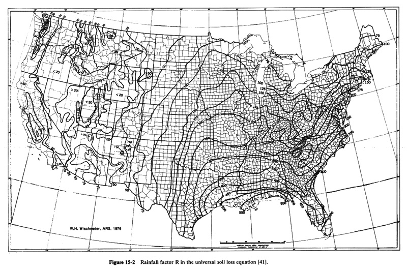
Rainfall factor
- When factors other than rainfall are held constant, soil losses from cultivated fields are shown to be directly proportional
to the product of the storm's total kinetic energy E and its maximum 30-minute intensity I.
- The product EI reflects the combined potential of raindrop impact and runoff turbulence to transport dislodged soil particles.
- The sum of EI products for a given year is an index of the erosivity of all rainfall for that year.
- The rainfall factor R is the average value of the series of annual sums of EI products.
- Values of R applicable to the contiguous United States are shown in Fig. 15-2.
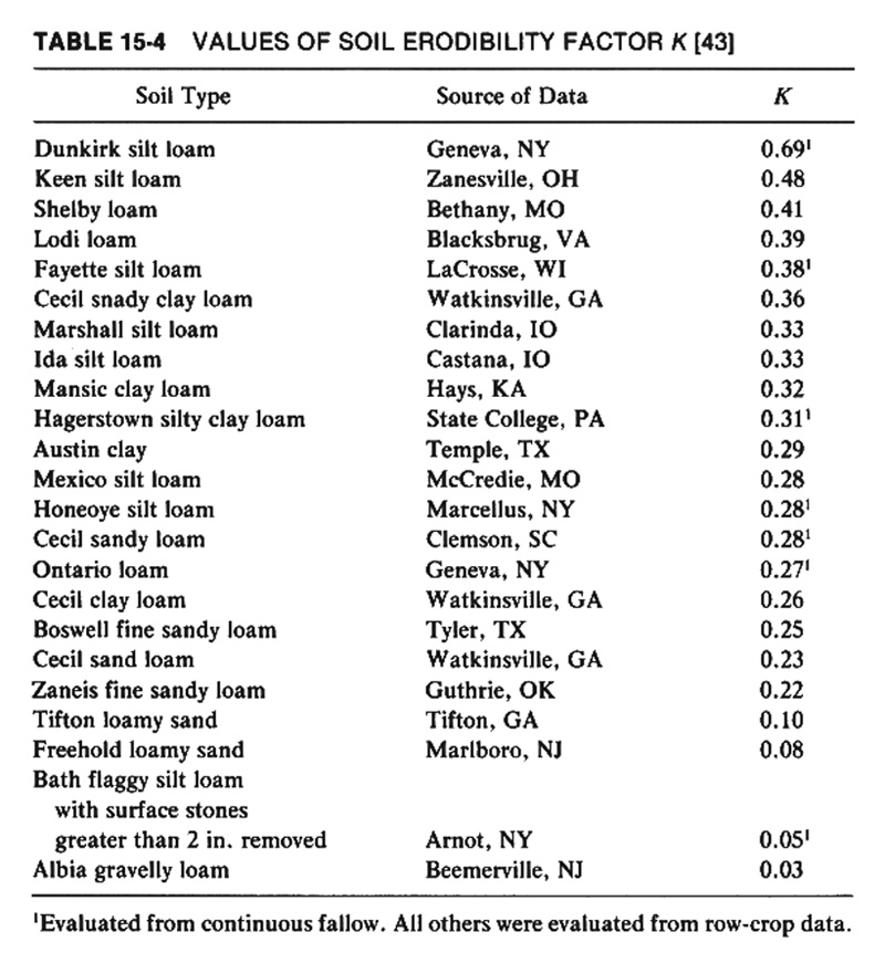
Soil erodibility factor
- The soil erodibility factor is a measure of the resistance of a soil surface to erosion.
- Its is defined as the amount of soil loss, in tons per acre per year, per unit of rainfall factor R for a unit plot.
- A unit plot is 72.6 ft long, with a uniform lengthwise gradient of 9%, in continuous fallow, tilled up and down the slope.
- Values of K for 23 major soils are shown in Table 15-4.
- K factors for other soils are estimated by comparison with those values in Table 15-4.
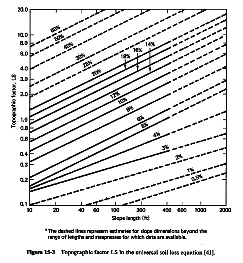
Slope-length and slope-gradient factors
- The rate of soil erosion by flowing water is a function of slope length (L) and gradient (S).
- For practical purposes, these two topographic characteristics are combined into a single topographic factor (LS).
- The factor LS is defined as the ratio of soil loss from a slope of given length and gradient to the soil loss from a unit plot of 72.6 ft length
and 9% gradient.
- Values of LS are shown in Fig. 15-3.
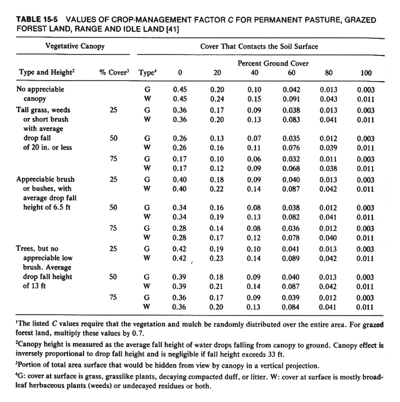
Crop management factor
- The crop management factor C is defined as the rate of soil loss from a certain combination of vegetative cover and management practice
to the soil loss resulting from tilled, continuous fallow.
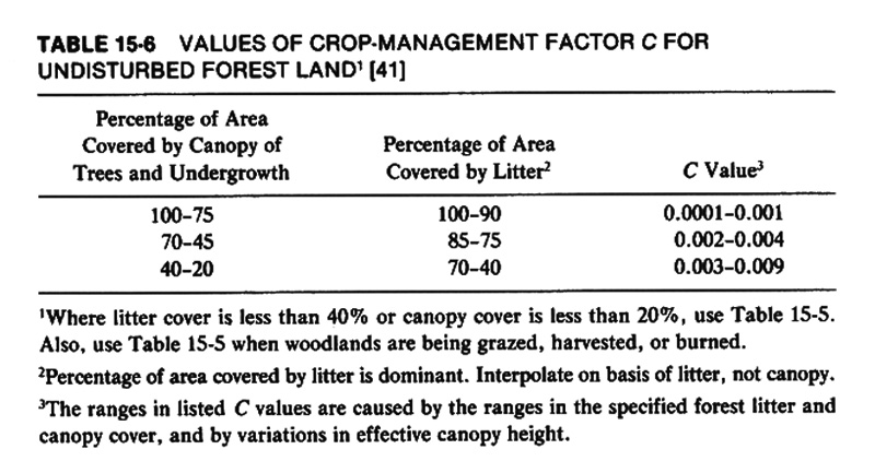
- Values of C range from as little as 0.0001 for undisturbed forest land to a maximum of 1 for disturbed areas with no vegetation.
- Values of C for cropland are estimated on a local basis.
- Values of LS are shown in Tables 15-5 and 15-6.
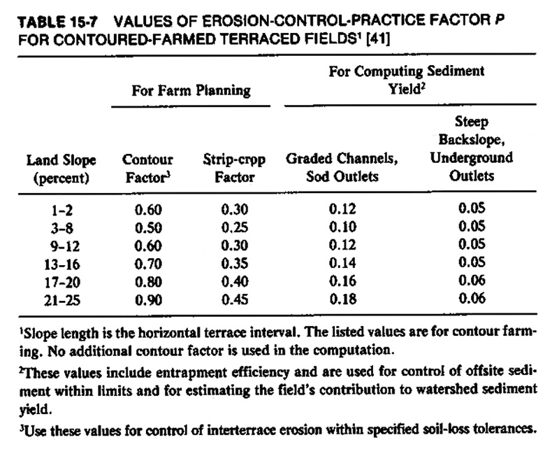
Erosion control practice factor
- The erosion control practice factor is defined as the ratio of soil loss under a certain erosion-control practice to the soil loss
resulting from straight row farming.
- Values of P have been established for contouring and contour strip cropping.
- In contour strip cropping, strips of sod or meadow are alternated with strips of row crops or small grains.
- Values of P used for contour strip cropping are also used for contour-irrigated furrows.
- Values of P are shown in Table 15-7.
Use of the Universal Soil Loss Equation
- The USLE cannot be used to compute sediment yield.
- For instance, for a 1000-km2 basin, only 5% of the soil loss computed by the USLE
may appear as sediment yield at the basin outlet.
- The remaining 95% is redistributed on uplands or flood plains, and it does not constitute a net loss from the drainage basin.
Example 15-3.
Assume a 600-ac watershed in Fountain County, Indiana.
Compute the average annual soil loss by the USLE for the following conditions:
- Cropland, 280 ac, contour strip-cropped, soil is Fayette silt loam, slopes are 8% and 200 ft long;
- Pasture, 170 ac, 50% canopy cover, 80% groundcover with grass, soil is Fayette silt loam, slopes are 8% and 200 ft long;
- Forest, 150 ac, soil is Marshall silt loam, 30% canopy cover, slopes are 12% and 100 ft long.
Solution:
-
From Fig. 15-2, R = 185
From Table 15-4, K = 0.38
From Fig. 15-3, LS = 1.4
Value of C for cropland is obtained from local sources. Assume C = 0.12
From Table 15-7, P = 0.25
A = R K SL C P = 2.95 tons/ac/yr
From Fig. 15-2, R = 185
From Table 15-4, K = 0.38
From Fig. 15-3, LS = 1.4
No value of P has been established for pasture. Assume P = 1.
A = R K SL C P = 1.18 tons/ac/yr
- From Fig. 15-2, R = 185
From Table 15-4, K = 0.33
From Fig. 15-3, LS = 1.8
No value of P has been established for pasture. Assume P = 1.
A = R K SL C P = 0.66 tons/ac/yr
The total sheet and rill erosion from the 600-ac watershed is:
(280 × 2.95) + (170 × 1.18) + (150 × 0.66) = 1126 tons/yr
Example 15-3 Online.
Verify this example with online usle 2.
[Watershed] soil loss = 1126.406 tons/yr
Channel erosion
- Channel erosion includes gully erosion, streambank erosion, streambed degradation, floodplain scour, and other sources of sediment,
excluding upland erosion.
- Gullies are incipient channels in process of development.
- Gully growth is usually accelerated by several climatic events, improper land use, or changes in stream base levels.
- Significant gully activity is found in regions of moderate to steep topography with thick soil mantles.
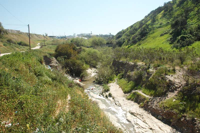
- Camp Creek, Oregon.
- The total sediment outflow from gullies is usually less than sheet and rill erosion.
- Streambank erosion and streambed degradation can be significant in certain cases.
- Downstream of a newly constructed dam, "hungry" water will cause streambed degradation.
Degradation to bedrock downstream of a sediment retention dam.
|
|
- Changes in channel alignment and/or removal of natural vegetation from streambanks may cause streambank erosion.
- Methods for determining soil loss due to various types of channel erosion include the following:
- Comparing aerial photos taken at different times,
- Performing river cross sectional surveys to determine changes in cross section,
- Assembling historical data,
- Performing field studies to evaluate annual growth.
- Field surveys may provide sufficient data to estimate streambank erosion as follows:
in which:
S = annual volume of streambank erosion,
H = average height of bank,
L = length of eroded bank, and
R = annual rate of bank recession (net rate).
- Streambed degradation can be estimated as follows:
in which:
S = annual volume of streambed degradation,
W = average bottom width of degrading channel reach,
L = length of degrading channel reach, and
R = annual rate of streambed degradation.
Accelerated erosion due to strip mining and construction activities
- Strip mining and construction activities greatly accelerate erosion rates.
- Human induced land distrubances have a substantial impact on sediment production.
- EPA's Best Management Practices (BMP's) are used to control erosion from anthropogenically disturbed sites.
- The USLE may be used to compute erosion from disturbed sites.
Sediment yield
- In engineering applications, the quantity of sediment eroded at the sources is not as important as the quantity of sediment delivered
to a downstream point, i.e., the sediment yield.
- Sediment yield is calculated by multiplying the gross sediment production by a sediment delivery ratio that varies in the range 0-1.
Sediment delivery ratio
- The sediment delivery ratio (SDR) is largely a function of:
- sediment source,
- proximity of sediment source to the fluvial transport
system,
- density and condition of the fluvial transport system,
- sediment size and texture, and
- catchment characteristics.
- The sediment source has an influence on the SDR.
- Not all sediments originating in sheet and rill erosion are likely to enter the transport system.
- Sediments originating in channel bank erosion are more likely to be delivered to downstream points.
- The amount of sediments delivered to downstream points will depend on the ability of the fluvial transport system to entrain and hold on to the sediment
particles.
- Silt and clay particles can be transported much more readily than sand particles.
- High catchment relief often indicates both high erosion and high SDR.
- High channel density is an indication of an efficient transport system and, therefore, of a high SDR.
Estimation of sediment delivery ratios
- The SDR is the ratio of sediment yield to gross sediment production.
- Estimates of sediment yield can be obtained by reservoir sedimentation surveys.
- Alternatively, sediment yield can be evaluated by a direct measurement of sediment load at the point of interest.
- Estimates of gross sediment production can be obtained with the USLE.
- When warranted, this estimate can be augmented by field measurements of gully and channel erosion.
- Regional SDR equations can be derived with data.
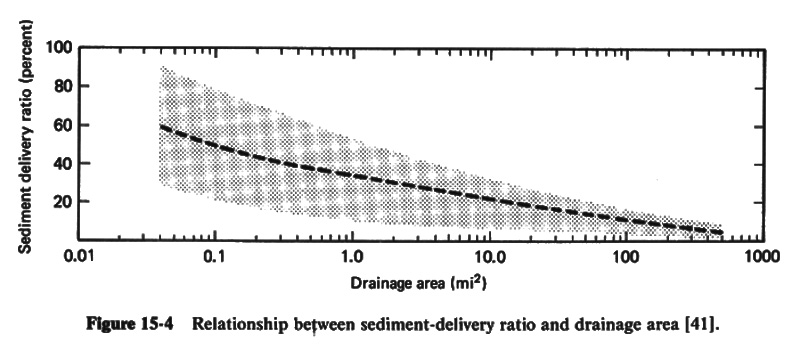
- The simplest SDR prediction equation is based solely on drainage area, as shown in Fig. 15-4.
- This figure shows that SDR varies in inverse proportion of the 1/5 power of the drainage area.
- The greater the drainage area, the smaller the catchment relief, and the greater the chances for sediment deposition within the catchment.
- Rough estimates can be obtained from Fig. 15-4, but caution is recommended for more detailed studies.
- An example of a regional SDR equation:
|
SDR = 31,623 (10 A)-0.23(L/R)-0.51 B-2.79
|
in which:
SDR = sediment delivery ratio,
A= drainage area, in sq. mi.,
L/R = ratio of catchment length to relief,
B = weighted mean bifurcation ratio, defined as the ratio of number of streams of a given order to the number of streams in the next higher order.
Empirical formulas for sediment yield
- Statistical analysis has been used to develop regional equations for the prediction of sediment yield.
- The Dendy and Bolton formula is a good example of a sediment yield equation.
Sediment yield vs drainage area
- Dendy and Bolton studied sedimentation data for about 1500 reservoirs, ponds, and detention basins.
- They used reservoirs with drainage areas greater than 1 sq mi.
- For drainage areas between 1 and 30,000 sq mi, Dendy and Bolton found that the annual sediment yield per unit area was inversely related to the 0.16 power
of the drainage area:
in which:
S = sediment yield in tons per acre per sq mi,
SR = reference sediment yield corresponding to 1 sq mi area, equal to 1645 tons/yr,
A = drainage area in sq mi, and
AR = reference drainage area, equal to 1 sq mi.
Sediment yield vs mean annual runoff
- Dendy and Bolton studied sedimentation data from 505 reservoirs having mean annual runoff data.
- Annual sediment yield per unit area was shown to increase sharply as mean annual runoff Q increased from 0 to 2 in.
- Thereafter, for mean annual runoff from 2 to 50 in, annual sediment yield per unit area decreased exponentially.
- This lead to the following equations for sediment yield:
For Q ≤ 2 in:
For Q > 2 in:
|
S/SR = 1.19 e -0.11(Q/QR)
|
in which:
QR = reference mean annual runoff, equal to 2 in.
- Dendy and Bolton further combined the equations for sediment yield in terms of drainage area and mean annual runoff into the following:
For Q ≤ 2 in:
|
S/SR = 1.07 (Q/QR)0.46 [1.43 - 0.26 log(A/AR)]
|
For Q > 2 in:
|
S/SR = 1.19 e -0.11(Q/QR) [1.43 - 0.26 log(A/AR)]
|
- For SR = 1645 tons/yr, QR = 2 in, and AR = 1 sq mi, the Dendy and Bolton equations reduce to:
For Q ≤ 2 in:
|
S = 1280 Q0.46(1.43 - 0.26 log A)
|
For Q > 2 in:
|
S = 1965 e -0.055Q (1.43 - 0.26 log A)
|
with Q in in., A in sq. mi., and S in tons/sq. mi./yr.
- These equations should be used with caution.
- In certain cases, local factors such as soils, geology, topography, land use, and vegetation may have a greater influence on sediment yield
than either mean annual runoff or drainage area.
Example 15-4.
Calculate the sediment yield by the Dendy and Bolton formula for a 150-sq mi watershed with 3.5 in of mean annual runoff.
Solution:
The application of the Dendy and Bolton formula leads to:
S = 210,000 tons/yr.
Example 15-4 Online.
Verify Example 15-4 with online dendy and bolton.
Sediment yield = 210,123.47 tons/yr.
Go to Lecture 17B.
|