|
|
CIVE 445 - ENGINEERING HYDROLOGY
CHAPTER 9D: STREAM CHANNEL ROUTING, MUSKINGUM-CUNGE METHOD
|
|
9.4 MUSKINGUM-CUNGE METHOD
|
- The Muskingum method can calculate runoff diffusion by varying the parameter X.
- A numerical solution of the linear kinematic wave equation using a third-order accurate scheme (C = 1) leads to pure flood hydrograph
translation (see Example 9-3, part 1).
- Other numerical solutions of the linear kinematic wave equation invariably produce a certain amount of
numerical diffusion and/or dispersion (see Example 9-3, part 2).
- The Muskingum and linear kinematic wave solutions are strikingly similar.
- The kinematic wave equation cannot properly describe physical diffusion.
- The diffusion wave equation can describe physical diffusion.
- From these propositions, Cunge correctly concluded the following:
- The Muskingum method is a linear kinematic wave solution.
- The flood wave attenuation shown by the calculation is due to the numerical diffusion of the scheme itself.
- Discretization of the kinematic wave equation.
- Discretization of the kinematic wave equation (continued).
- The routing coefficients are a function of X and C.
- It is seen that by defining K = Δx/c, the Muskingum and Muskingum-Cunge routing coefficients are the same.
- This confirms that K is indeed the flood-wave travel time: the time it takes a given discharge to travel the reach length Δx
with the kinematic wave celerity c.
- The celerity c can be assumed to be constant (linear mode) or to vary with discharge (nonlinear mode).
- For X= 0.5, these equations are the same as the second-order linear kinematic wave solution.
- For X = 0.5 and C = 1, the routing equation is third-order accurate. i.e., exact.
- For X = 0.5 and C ≠ 1 it is second-order accurate, exhibiting only numerical dispersion (dips in the calculated hydrograph).
- For X < 0.5 and C ≠ 1 it is first-order accurate, exhibiting both numerical diffusion and dispersion.
- For X < 0.5 and C = 1 it is first-order accurate, exhibiting only numerical diffusion.
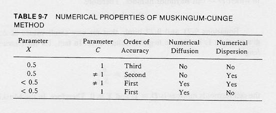
Table 9-7
|
- The best way to use the Muskingum-Cunge method is to set X < 0.5 and C = 1 (only numerical diffusion).
- The numerical diffusion can be used to simulate the physical diffusion of the flood wave.
- By expanding the discrete function Q(jΔx, nΔt), in Taylor series about grid point (jΔx, nΔt),
the numerical diffusion coefficient of the Muskingum-Cunge scheme is derived (Appendix B):
- In which νn is the numerical diffusion coefficient of the Muskingum scheme.
- This equation reveals the following:
- For X = 1/2, there is no numerical diffusion, although there is numerical dispersion for C ≠ 1.
- For X > 1/2, the numerical diffusion coefficient is negative, i.e., numerical amplification, which explains the behavior
of the Muskingum method when X > 0.5 (dips).
- For Δx = 0, the numerical diffusion coefficient is zero, clearly the trivial case.
- A predictive equation for X can be obtained by matching the hydraulic diffusivity νh with the numerical diffusivity
νn.
- This leads to the following expression for X:
|
X = (1/2) { 1 - [qo/(So c Δx)]}
|
- With X calculated with this equation, the Muskingum method is referred to as Muskingum-Cunge method.
- In this way, the routing parameter X can be calculated as a function of the following physical and numerical properties:
- reference discharge per unit width qo;
-
bottom slope So;
- kinematic wave celerity c;
- reach length Δx.
- It is noted that matching physical and numerical diffusion does not control numerical dispersion.
- Therefore, for the method to work correctly, it is necessary to optimize numerical diffusion (by calculating X)
while minimizing numerical dispersion (by keeping C as close to 1 as possible)
- A unique feature of the Muskingum-Cunge method is the grid independence of the calculated outflow hydrograph.
- This sets it apart from other methods such as the convex method, which feature uncontrolled numerical diffusion and dispersion.
- If numerical dispersion is minimized, the calculated outflow at the downstream end of a channel reach
will be the same, regardless of how many subreaches are used in the computation.
- In other words, the results are independent of the grid size.
- An improved version of the Muskingum-Cunge method is the following,
adopted by HEC-1 in 1990 and HEC-HMS in 1998.
- The Courant number is:
- The grid diffusivity is defined as the numerical diffusivity for X = 0:
- The cell Reynolds number is defined as the ratio of hydraulic diffusivity to grid diffusivity:
- Therefore:
- For very short reaches (Δx small), D may be greatewr than 1, and X less than 0.
- For the characteristic reach length:
- It follows than D = 1 and X = 0.
- In the Muskingum-Cunge method, reach lengths shorter than Δxc
result in negative values of X.
- This should be contrasted with the Muskingum method, where X is restricted in the range 0.0-0.5.
- In the Muskingum method, X is interpreted as a weighting factor.
- Nonnegative values of X are associated with long reaches, typical of the manual computation used in the development and early application
of the Muskingum method.
- In the Muskingum-Cunge method, X is interpreted in a moment-matching sense or diffusion matching factor.
- Therefore, negative values of X are entirely possible.
- This allows the use of short reaches (in the computer-aided calculation).
- The substitution of C and D into the routing equations of the Muskingum-Cunge method leads to:
|
C0 = (-1 + C + D) / (1 + C + D)
|
|
C1 = (1 + C - D) / (1 + C + D)
|
|
C2 = (1 - C + D) / (1 + C + D)
|
- The calculation of the routing parameters can be performed in many ways.
- For natural cross-sections, it is always better to base the kinematic wave celerity c on the geometric and hydraulic properties of the
cross-section.
- The calculations can proceed in a linear or nonlinear mode.
- In the linear mode, the routing parameters are based on predetermined reference flow values.
- The choice of reference flow values has a bearing on the results, but the effect is likely to be small.
- In the nonlinear mode, the routing parameters are varied with the flow, i.e., for each computational grid cell.
- The constant-parameter method resembles the Muskingum method, with the addition of physically based parameters.
- The variable-parameter method resembles more advanced routing methods such as the dynamic wave.
- Example 9-9.
- Example 9-9 (continued).
- The values Δx and Δt should be sufficiently small.
- C + D should be greater than 1.
- C should be around 1 to minimize numerical dispersion.
- In practice, C should be restricted between 1 and 2.
Assessment of the Muskingum-Cunge method
- The Muskingum-Cunge method is a physically based alternative to the conceptual/empirical Muskingum method.
- In the Muskingum method, the parameters are calibrated using streamflow data (hydrology).
- In the Muskingum-Cunge method, the parameters are based on flow and channel characteristics (hydraulics).
- This makes possible channel routing without the need for calibration.
- It makes possible channel routing in ungaged streams.
- With the variable-parameter method, nonlinear properties of flood waves can be described within the context of the Muskingum formulation.
- Like the Muskingum method, the Muskingum-Cunge method is limited to diffusion waves.
- The Muskingum-Cunge method is suited for channel routing of kinematic and diffusion waves
in natural streams without significant backwater effects.
- It is noted that the Muskingum method is based on the storage concept (Chapter 4), and that the parameters K and X
are reach averages.
- However, the Muskingum-Cunge method is
kinematic in nature, with parameters C and D based on hydraulic values evaluated at channel cross
sections.
- Thus, for the Muskingum-Cunge method to improve on the Muskingum method, it is necessary that the routing parameters evaluated at channel cross sections be representative of the reach storage properties.
- The Muskingum method follows storage concept, and is based on historic (hydrologic) data. If there is no historic data,
it cannot be applied in a predictive mode.
- The Muskingum-Cunge method follows kinematic wave theory, and is based on geometric and hydraulic data.
- This data can be measured for an individual reach at any time,
without having to wait for the flood to occur.
- The Muskingum-Cunge method is better suited to distributed computation (current hydrologic modeling).
- This is why the Muskingum-Cunge method has been adopted by the Corps of Engineers'
HEC-1 and HEC-HMS.
|
9.5 INTRODUCTION TO DYNAMIC WAVES
|
- Kinematic waves were formulated by simplifying the momentum conservation principle to a statement of steady uniform flow.
- Diffusion waves were formulated by simplifying the momentum conservation principle to a statement of steady nonuniform flow.
- These two waves have been amply used in stream channel routing applications.
- The Muskingum and Muskingum-Cunge methods are examples of the application of diffusion waves.
- The dynamic wave is formulated taking into account the complete momentum principle, including inertia.
- The dynamic wave contains more physical information that either kinematic or diffusion waves.
- Dynamic wave solutions are more complex than kinematic and diffusion wave solutions.
- In a dynamic wave solution, the equations of mass and momentum conservation are solved by a numerical procedure, either finite
differences, finite elements, or the method of characteristics.
- In the past 20 years, the method of finite differences is the preferred way of obtaining a dynamic wave solution.
- The Preissmann numerical scheme is most popular.
- This is four-point scheme, centered in the temporal derivative and slightly offcentered in the spatial derivative.
- This offcentering is necessary to control the numerical stability of the nonlinear scheme.
- This produces a stable yet workable scheme.
- The application of the Preissmannn scheme to the governing equations for the various reaches results in a matrix solution
requiring a double-sweep algorithm.
- A dynamic wave solution represents an order-of-magnitude increase in complexity and associated data requirements.
- Its use is recommended when kinematic or diffusion waves are not applicable, i.e., for dam-breach routing or routing near tidal
situations.
- It is recommended for cases warranting a precise determination of the unsteady variation of river stages.
- Therefore, it remains a hydraulic method.
Relevance of Dyamic Waves to Enginering Hydrology
- Dynamic wave solutions are often referred to as hydraulic river routing.
- Kinematic waves calculate unsteady discharges; the corresponding stages, if needed, are later obtained from the appropriate rating curves.
- Usually, equilibrium (steady, uniform, unique) rating curves are used for the purpose of converting discharge to stage.
- Dynamic waves rely on the physics of the phenomena, as built into the governing equations, to generate their own unsteady rating.
- A looped rating is produced at every cross section (see Figure 9-9).

Fig. 9-9
|
- This loop is due to hydrodynamic reasons; it should not be confused with other loops which may be due to erosion, sedimentation, or changes
in bed configuration.
- The width of the loop is a measure of the flow unsteadiness; wider loops corresponding to highly unsteady flows, i.e., dynamic waves.
- If the loop is narrow, the wave may be a diffusion wave.
- If the loop is practically nonexistent, the wave is a kinematic wave.
- In fact, the basic assumption of kinematic waves is that the rating curve is single-valued (unique).
- The relevance of dynamic waves in engineering hydrology is directly related to the amount of flow unsteadiness and the associated loop in the
rating curve.
- For highly unsteady flows, such as dam breaches, it may be the only way to properly account for the loop in the rating.
- Dam breach flood waves are know to be very diffusive, i.e., dynamic.
- Example: Teton Dam, in Idaho,
that failed in June 1975, releasing 1,700,000 cfs, which were measured about 100 miles downstream as 50,000 cfs
(attenuation to 3% of original flow).
Diffusion wave solution with dynamic component
- A simplified approach to dynamic wave routing is that of the diffusion wave with dynamic component.
- In this approach, the complete goiverning equations, including inertia terms, are linearized in a similar way as with diffusion waves.
- This leads to a diffusion wave equation, but with a modified hydraulic diffusivity:
|
∂Q/∂t + [∂Q/∂A] (∂Q/∂x) = [Qo/(2TSo)] [1 - (β - 1)2Fo2] ∂2Q/∂2x
|
- in which the Froude number is:
- The quantity (β-1)Fo has now been recognized as the Vedernikov number.
- With this addition, the governing equation is able to include the dynamic effect.
- For instance, for β= 3/2, and F = 2, the hydraulic diffusivity vanishes, which is in agreement with physical reality.
- The hydraulic diffusivity of the diffusion wave is independent of the Froude number.
- Including the Froude-number dependence of the hydraulic diffusivity increases the range of applicability of the diffusion wave to
flows near and above critical.
- However, most natural flows are well below critical state, and the diffusion wave remains widely applicable.
Go to
Chapter 10A.
|