|
|
CIVE 445 - ENGINEERING HYDROLOGY
CHAPTER 10A: CATCHMENT ROUTING, TIME-AREA METHOD
|
- Catchment routing refers to the calculation of flows in time and space within a catchment.
- The objective of catchment routing is to transform effective rainfall into streamflow.
- This is accomplished either in:
- Lumped mode: time-area method
- Distributed mode: kinematic wave method
- Methods of catchment routing are similar to those of reservoir and stream channel routing.
- In fact, many techniques used in reservoir and channel routing are also applicable to catchment routing.
- Kinematic wave techniques were originally developed for river routing, but were later applied
to catchment routing.
- Methods of catchment routing are of two types:
- Hydrologic
- Hydraulic
- Hydrologic methods are spatially lumped to provide a runoff
hydrograph at the catchment outlet.
- Examples of hydrologic routing methods are:
- The time-area method (TAM) and
- The cascade of linear
reservoirs (CLR).
- Hydraulic routing uses kinematic and diffusion waves to simulate surface runoff within a
catchment in a distributed context.
- Catchment routing can use parametric, conceptual, and/or deterministic components.
- For instance, the hydrograph obtained by the time-area method can be routed through a
linear reservoir using a storage constant K derived by
empirical means.
- The cascade of linear reservoirs is a typical example of a conceptual model used in catchment routing.
- Kinematic and diffusion models are examples of deterministic methods used in catchment routing.
- The concepts of translation and storage
are central to the study of flow routing.
- Unlike in reservoir and
stream channel routing, translation and storage can be studied separately in catchment routing.
- Translation is interpreted as the movement of water in a direction parallel to the channel bottom.
- Storage is interpreted as the movement of water in a direction perpendicular to the channel bottom.
- Translation is synonymous with runoff concentration.
- Storage is synonymous with runoff diffusion.
- In reservoir routing, storage is the primary mechanism, with translation almost nonexistent.
- In stream channel routing, translation is the predominant mechanism (first order),
while storage is secondary (second order).
- This is why kinematic and diffusion models are useful models of stream channel routing.
- In catchment routing, translation and storage are about equally important.
- This is why they are often accounted for separately.
- The translation effect is related to runoff concentration,
while the storage effect can be simulated with linear reservoirs.
- The time-area method of hydrologic catchment routing transforms an effective storm hyetograph
into a runoff hydrograph.
- The method accounts for translation only, and does not include storage.
- Therefore, hydrographs calculated by the time-area method show a lack of diffusion, resulting in higher
peaks that those that would have been obtained if storage had been taken into account.
- If necessary, the required amount of storage can be incorporated by routing the hydrograph obtained
by the time-area method through a linear reservoir.
- The required amount of storage is determined by calibrating the linear reservoir storage
constant K with measured data.
- Alternatively, suitable values of K can be estimated based on regionally derived formulas.
- The time-area method is essentially an extension of the runoff concentration principle used in the
rational method (Chapter 4).
- Unlike the rational method, however, the time-area method can account for the temporal variation
of rainfall intensity.
- Therefore, the applicability of the time-area method is extended to midsize catchments.
- The time-area method is based on the concept of time-area histogram.
- This is a histogram of contributing catchment subareas.
- To develop a time-area histogram:
- The catchment's time of concentration is divided into a number of equal time intervals.
- Cumulative time at the end of each time interval is used to divide the catchment into zones delimited
by isochrone lines, i.e., the loci of points of equal travel
time to the catchment outlet
[Fig. 10-1 (a)].
- The time intervals of the effective rainfall hyetograph and time-area histogram should be equal.
- The rationale for the time-area method is that, according to the runoff concentration principle
(Chapter 2),
the partial flow at the end of each time interval is equal to the product of effective rainfall
times contributing subarea:
Q = ieA
- The lagging and summation of the partial flows results in a runoff hydrograph for the given
effective rainfall hyetograph and time-area histogram.
- While the time-area method accounts for runoff concentration only, it has the advantage that the
catchment shape is reflected in the time-area histogram, and therefore, in the runoff hydrograph.
- Example 10-1
- Example 10-1:
Table 10-1
- It is readily seen that the time-area method and the rational method share a common theoretical basis.
- However, since the time-area method uses effective rainfall and does not rely on runoff coefficients,
it can account only for runoff concentration, with no provision for runoff diffusion.
- Diffusion can be provided by routing the hydrograph calculated by the time-area method through a linear
reservoir with an appropriate storage constant K.
- The time-area method leads to an alternate way of calculating time of concentration.
- Provided there is no runoff diffusion, as would be the case of a hydrograph calculated with the time-area
method, the time of concentration is the difference between hydrograph time base Tb
and effective rainfall duration tr.
- In other words, the time of concentration is
the time elapsed from the end of effective rainfall to the end of runoff.
- There is another way to express time of concentration, based on the measured hydrograph.
- This method assumes that the time to the
point of inflection ti (i.e., the point of
zero curvature) on the receding limb of a measured (i.e., translated and diffused) hydrograph coincides
with the time to the end of the translated-only hydrograph (Tb). Therefore:
- The advantage of this equation is the ti is readily ascertained, while Tb is not.
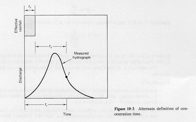
Fig. 10-3
|
|
10.2 CLARK UNIT HYDROGRAPH
|
The linear reservoir storage constant K can be calculated directly from the tail of a measured hydrograph.
To illustrate the procedure, in Table 10-2, Col. 9, the two lines for t = 6 h and t = 7 h show zero
outflow in the translated-only unit hydrograph, that is, zero inflow to the linear reservoir.
The average outflow (between t = 6 h and t = 7 h) (Col. 9) is:
|
O = (46.19 + 27.72) / 2 = 36.955 m3/s.
|
The rate of change of outflow (between t = 6 h and t = 7 h) (Col 9) is:
|
dO/dt = (27.72 - 46.19) / (1 h) = -18.47 (m3/s)/h.
|
Therefore, the storage constant is:
|
K = - [36.995/(-18.47)] = 2 h.
|
This equation applies at the tail of the outflow hydrograph, after the translated-only (outflow
hydrograph from
time-area method, inflow to linear reservoir)
has receded back to zero.
Alternatively, the Clark parameters (concentration time and linear reservoir storage constant)
can be estimated based on catchment characteristics.
|
10.3 CASCADE OF LINEAR RESERVOIRS (CLR)
|
- A linear reservoir has a diffusion effect on the inflow hydrograph.
- If an inflow hydrograph is routed through a linear reservoir, the outflow hydrograph has a reduced peak
and a longer time base.
- This increase in time base causes a difference in the relative timing of inflow and outflow
hydrographs, referred to as the lag.
- The amount of diffusion (and associated lag) is a function of the ratio Δt/K.
- Stronger diffusion effects correspond to smaller values of Δt/K.
- The cascade of linear reservoirs (CLR) is a widely used method of hydrologic catchment routing.
- The method is based on the connection of several linear reservoirs in series.
- For N such reservoirs, the outflow from the first would be taken as inflow to the second,
the outflow from the second would be taken as inflow to the third, and so on, until
the outflow from the (N-1)th would be taken as inflow to the Nth reservoir.
- The outflow from the Nth reservoir is taken as the outflow from the cascade.
- Although abstract, the cascade of linear reservoirs has proven to be useful in practice.
- Each reservoir in the series provides a certain amount of diffusion and associated lag.
- For a given set of parameters Δt/K and N, the outflow from the last reservoir is a function of
the inflow to the first reservoir.
- In this way, a one-parameter linear-reservoir method (Δt/K) is extended to a
two-parameter catchment routing method.
- Moreover, the basic linear-reservoir
routing formula
and routing coefficients remain essentially the same.
- The addition of a second parameter (N) provides considerable flexibility in simulating a wide range of
diffusion and associated lag effects.
- The conceptual basis of the method restricts its general use, since there is no relation
of either of the parameters to the physical diffusion of the catchment.
- The method has been used for large basins, where there is a substantial amount of stream-gaging data
to calibrate the parameters.
- Rainfall-runoff data can be used to determine the parameters Δt/K and N that produce the best fit
to the measured data.
- The analytical version of the cascade of linear reservoirs is referred to as the Nash model.
- The numerical (discrete) version is featured in several computer models developed in the
United States and other countries.
- Notable among them is the SSARR model, which uses it in its watershed and stream channel routing
modules.
- The routing equation of the cascade is the following:
|
Qj+1n+1 =
C0 Qjn+1 +
C1 Qjn +
C2 Qj+1n
|
- Fig. 10-4.
- The routing coefficients are:
- The routing parameter or Courant number C is:
- The average inflow is:
|
Qj (ave) =
(Qjn +
Qjn+1) / 2
|
- Substituting the average inflow into the routing equation leads to:
|
Qj+1n+1 =
2 C1 Qj (ave) +
C2 Qj+1n
|
- Alternatively, by adding and subtracting Qj+1n on the RHS:
|
Qj+1n+1 =
2C1 Qj (ave)
+ C2Qj+1n + Qj+1n - Qj+1n
|
|
Qj+1n+1 =
2C1 (Qj (ave) - Qj+1n)
+ Qj+1n
|
|
Qj+1n+1 =
[ 2C / (2 + C)] (Qj (ave) - Qj+1n)
+ Qj+1n
|
- This is the routing equation used in the U.S. Army Corps of Engineers' SSARR model.
- Smaller values of C lead to greater amounts of runoff diffusion.
- Values of C > 2 are not recommended, since they may lead to
negative diffusion (amplification).
- Example 10-3
- The cascade of linear reservoirs provides a convenient mechanism for simulating a wide range of catchment
routing problems.
- The method can be applied to each runoff component (surface runoff, subsurface runoff, and baseflow)
separately.
- The catchment response is taken as the sum of the responses of the individual components.
- For instance, assume a certain basin has 10 cm of runoff, of which 7 cm are surface runoff, 2 cm are
subsurface runoff, and 1 cm is baseflow.
- Since surface runoff is the less diffused process, it can be simulated with a high C = 1 and a
small number of reservoirs N = 3.
- Subsurface runoff is much more diffused than surface runoff; therefore,
it can be simulated with C = 0.4 and N = 5.
- Baseflow, being very diffused, can be simulated with C = 0.1 and N = 7.
- In practice, values of C and N are determined by extensive calibration.
- The cascade of linear reservoirs remains a conceptual model supported with empirical data.
- The method has been applied to large rivers such as the Upper Paraguay river
in Brazil,
the Salt river in Arizona, and the Mekong river in Thailand.
- The CLR is being used by the Hydrologic Research Center, a hydrologic firm in San Diego
for flood forecasting.
|