2.1 KINDS OF OPEN CHANNELS
The
- There are two kinds of channels:
- Artificial (prismatic)
- Natural (non-prismatic)
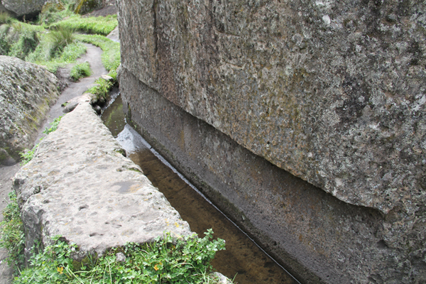
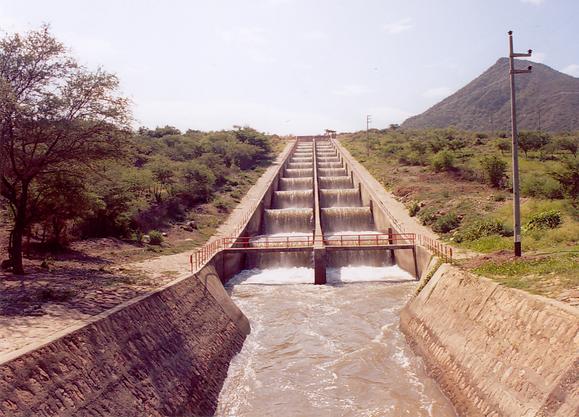
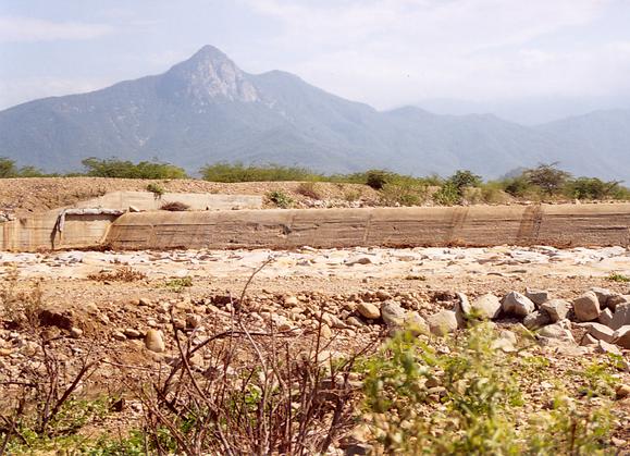
Tinajones feeder canal, Chiclayo, Peru
|
|
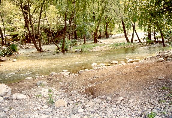
Rio La Silla Natural Park, Monterrey, Mexico.
|
|
- Other water-resources-related fields:
- Hydrology: the study of water in the hydrologic cycle.
- Hydroclimatology: the study of climate and the hydrologic cycle.
- Fluvial geomorphology: the study of the shape of streams and rivers.
- River mechanics: the study of the mechanical properties and behavior or rivers.
- Sedimentology: the study of sediment.
- Potamology: the study of rivers.
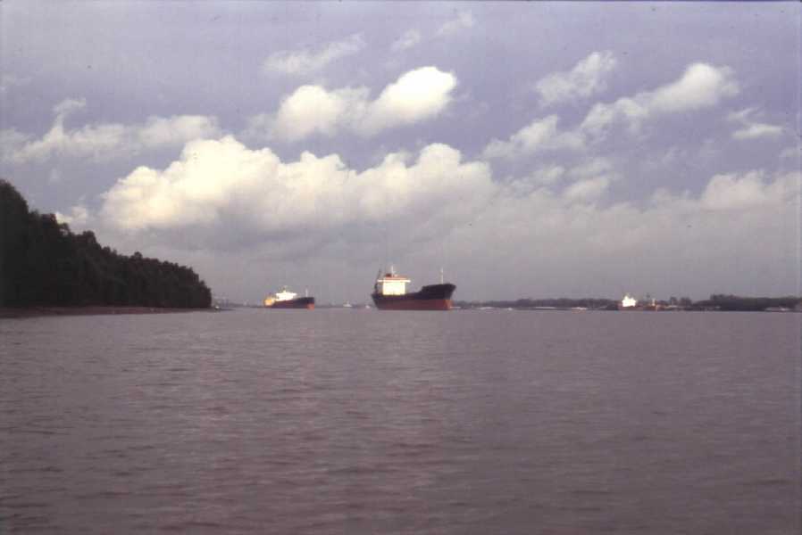
Lower Mississippi river near Baton Rouge, Louisiana.
|
|
- Uses of artificial channels:
- Navigation channels
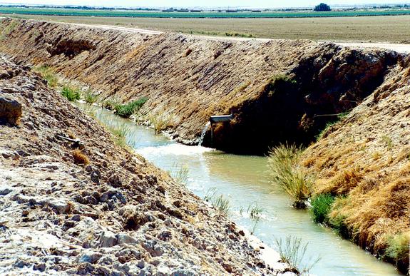
- Water conveyance channels (Example: the Dulzura conduit,
which links Barrett reservoir with drainage to Lower Otay reservoir, in San Diego County)
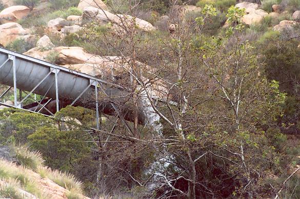
The Dulzura conduit, San Diego County, California.
|
|
- Power canals
- Irrigation canals (Example: the All-American canal, in the Imperial valley)
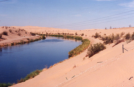
The All-American canal, Imperial County, California.
|
|
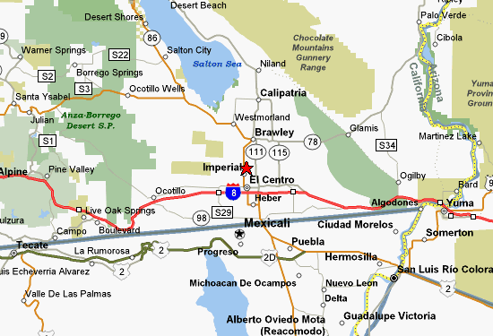
Location of the All-American canal, Imperial County, California.
|
|
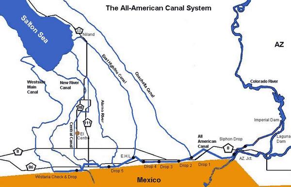
Location of the All-American canal, Imperial County, California.
|
|
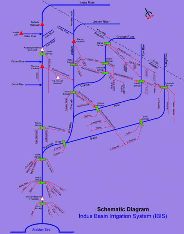
Indus Basin Link Canals, Pakistan.
|
|
- Flood control channels, floodways.
Rio Santa Catarina, Monterrey, Mexico.
|
|
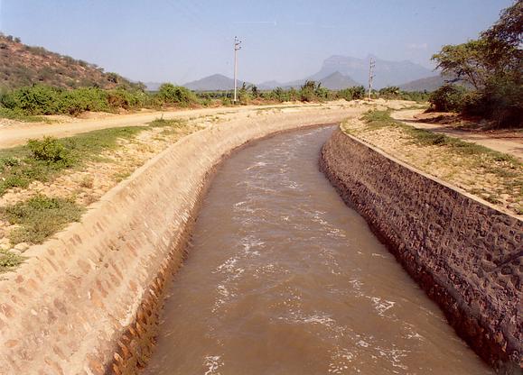
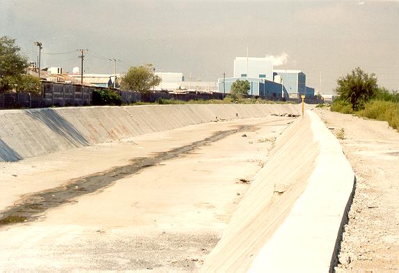
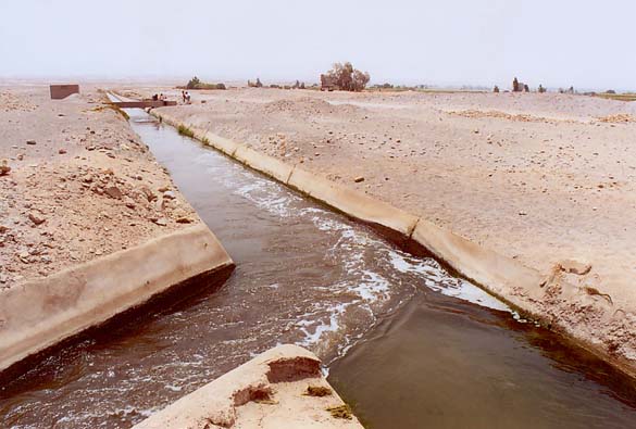
- Drainage ditches (drainage ditches in Imperial valley, draining to the Salton Sea).
Imperial Valley irrigation drain.
|
|
- Names for channels:
- Canal: long, mild-sloped, lined/unlined, ground-supported, masonry/concrete/wood/asphalt.
- Flume: supported above ground (lab flume), wood/metal/concrete/masonry.
- Chute: channel with steep slope, usually supercritical.
- Drop: Chute with very short distance.
- Culvert: covered channel of comparatively short length, flowing partially full.
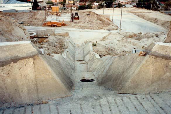
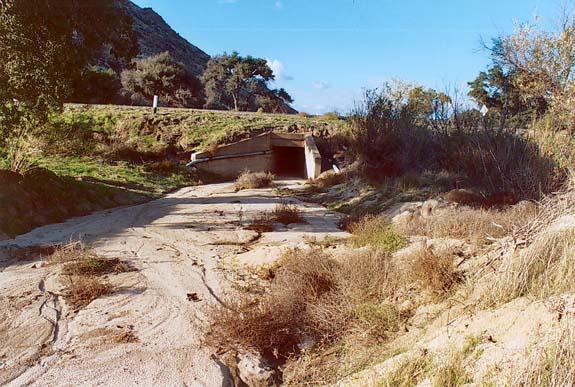
Drainage drop structure in Tijuana, Baja California.
|
|
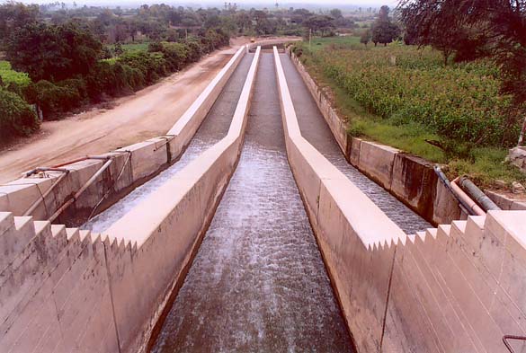
Tinajones drop structure, Chiclayo, Peru.
|
|
Chute at Taymi Canal, Chiclayo, Peru.
|
|
Canal with falls, La Joya, Arequipa, Peru.
|
|
Junction of main irrigation canal with main drain, La Joya, Arequipa, Peru.
|
|
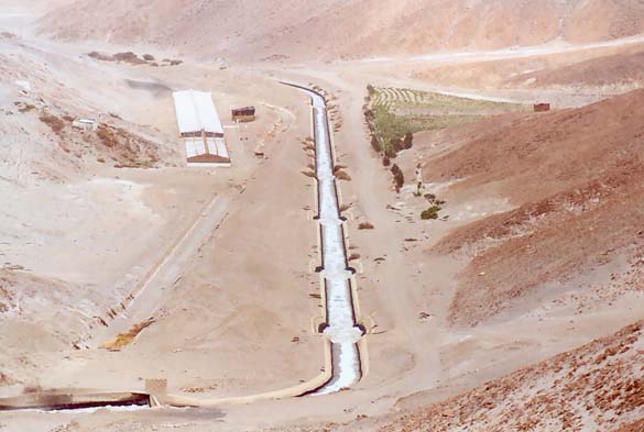
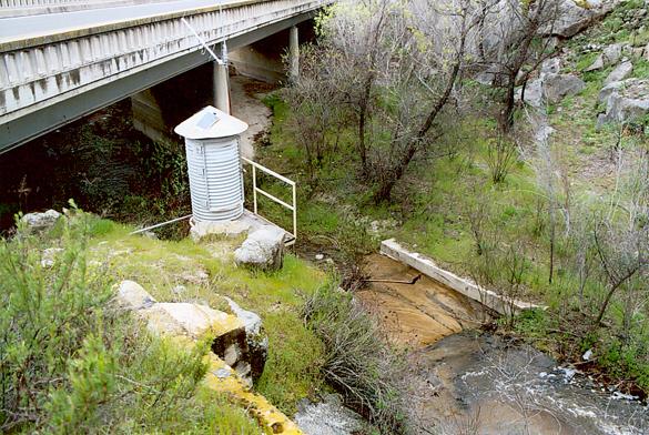
Crossing of Tinajones Feeder Canal with Chiriquipe Wash, Chiclayo, Peru.
|
|
Crossing of Arroyo Rosa de Castilla with Mexico Highway 2, Tecate, Baja, California.
|
|
2.2 CHANNEL GEOMETRY
The
- A prismatic channel has a constant cross section and constant bottom slope.
- The channel section is the cross section normal to the direction of flow.
- A trapezoid is the most common cross-sectional shape. It provides bank stability.
- A rectangular section is used in laboratory flumes.
- Channels built of stable materials (rock, concrete) can be rectangular.
- Triangular channels are used in ditches, roadside gutters.
- Depth of flow y: vertical distance from the free surface to the lowest point in channel cross section.
- Depth of flow section d: height of channel cross section; depth normal to direction of flow.
- For a channel with a longitudinal slope angle θ:
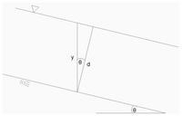
Fig. 2-9 (Chow)
|
|
- Stage y: elevation of the free surface.
- Top width T: width of channel cross section at free surface.
- Flow area A: area of flow in channel cross section.
- Wetted perimeter P: important in determining friction.
- Hydraulic radius R: ratio A/P.
- Hydraulic depth D: ratio A/T.
- For hydraulically wide channels: T ≈ P
- For hydraulically wide channels: D ≈ R
- In a channel section, the velocities near the surface and near the bottom differ.
- Velocities near the boundary are close to zero (no-slip condition).
- Large velocity gradients near the boundary produce large shear stresses
(which entrain and transport sediment).
- The maximum velocity occurs near the surface, at a distance of 0.05 to 0.25 of the flow depth.
- Velocities also vary transversally along horizontal bends; they are larger on the outside of the bend.
- Channel roughness will cause the curvature of the vertical velocity profile to increase.
- In a wide open channel, the sides have no influence on the velocity profile.
- The flow has a tendency to be 2-D instead of 3-D.
- Ratio T/D > 10 will assure wide-channel condition.
- Often a hydraulic analysis is carried out per unit of channel width.
- In a rectangular channel:
2.3 VELOCITY DISTRIBUTION
The
2.4 MEASUREMENTS OF VELOCITY
The
- Measurements are taken with a current meter positioned at 0.6 d, measured from the surface.
- Also, at 0.2 d and 0.8 d, and then find the average of these two values.
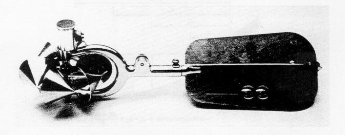
Price AA current meter (Courtesy of the U.S. Geological Survey).
|
|
USGS gaging stating at Campo Creek, San Diego County, California.
|
|
2.5 VELOCITY DISTRIBUTION COEFFICIENTS
The
- Due to nonuniform distribution of velocities over a cross section, the true velocity head is usually greater than the value
computed based on the mean (average) velocity.
- The true velocity head is:
- α is the energy coefficient or Coriolis coefficient.
- The value of α is typically in the range 1.03-1.36 for fairly straight prismatic channels.
- The value is greater for small channels, and smaller for large channels.
- The true momentum flux is:
- β is the momentum coefficient or Boussinesq coefficient.
- The value of β is typically in the range 1.01-1.12 for fairly straight prismatic channels.
- The values of α and β are slightly greater than 1.
- α is always greater than β.
- In channels of complex cross section, the values of α and β can easily get to be 1.6 and 1.2, respectively.
- Values of α greater than 2 have been observed in very irregular cross sections.
- The true velocity head is usually greater than the value
computed based on the average velocity.
- Assume:
- A = total area of the cross section [L2]
- ΔA = incremental area [L2]
- Vm = mean velocity of the cross section [L T-1]
- V = velocity through ΔA [L T-1]
- The weight flux through ΔA is:
- The weight flux through A is:
- Kinetic energy = force × distance = (mass × acceleration) × distance = (1/2) mV2 [M L2 T-2]
- Momentum = force × time = (mass × acceleration) × time = mV [M L T-1]
- Velocity head = kinetic energy per unit of weight
- Velocity head = [(1/2) m V2] / (mg) = V2/(2g) [L]
- Kinetic energy flux [through incremental area ΔA] =
kinetic energy per unit of weight × weight flux =
[V2/(2g)] [γ V ΔA]= γ V3 ΔA /(2g)
- For all the increments of area ΔA:
∑ γ V3 ΔA /(2g)
- Kinetic energy flux [through total area A] =
kinetic energy per unit of weight × weight flux =
[αVm2/(2g)] [γ Vm A] = α γ Vm3 A /(2g)
- Therefore:
∑ V3 ΔA = α Vm3 A
- Momentum β coefficient:
- The mass flux through ΔA is:
- The mass flux through A is:
- Momentum = force × time = mass × velocity = m V [M L T-1]
- Momentum flux = mass flux × velocity [F]
- The momentum flux through ΔA is:
- For all the increments of area ΔA:
∑ ρ V2 ΔA
- The momentum flux through A is:
- Therefore:
∑ V2 ΔA = β Vm2 A
- Energy flux = (weight flux) × (velocity head) [(F/T) L = FL/T]
- Momentum flux (force) = (mass flux) × (velocity) [(M/T) (L/T) = M (L/T2)]
- Note that the mean velocity is defined as:
- For approximate values, α and β can be computed as follows:
with
2.6 PRESSURE DISTRIBUTION
The
- The pressure is measured by the height of the water column at any point in the vertical.
- The pressure at any point is directly proportional to the depth of the point and equal to the hydrostatic pressure
corresponding to this depth.
- The distribution is linear, and is known as the hydrostatic law of pressure distribution.
- This assumes no vertical accelerations.
- This type of flow is known as parallel flow.
- The streamlines have no substantial curvature.
- Uniform flow is practically parallel flow.
- Gradually varied flow may be regarded as parallel flow.
- If the curvature is substantial, the flow is curvilinear flow.
- In curvilinear flow, the pressure distribution is not hydrostatic.
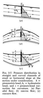
Fig. 2-7 (Chow)
|
|
- The centrifugal pressure p is [mass (per unit of area) × centrifugal acceleration]:
- The pressure rise c is:
- The rise is positive for concave flow, and negative for convex flow.
QUESTIONS
PROBLEMS
REFERENCES
Chow, V. T. 1959. Open-channel Hydraulics. McGraw Hill, New York.
| http://openchannelhydraulics.sdsu.edu |
|
140602 10:15 |