|
|
|
CHAPTER 2: PROPERTIES OF OPEN CHANNELS |
2.1 KINDS OF OPEN CHANNELS
|
|
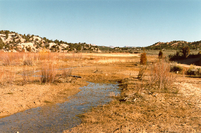
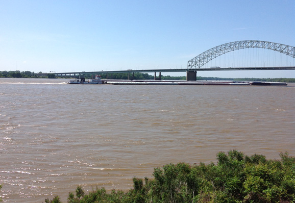
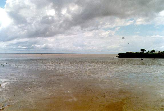
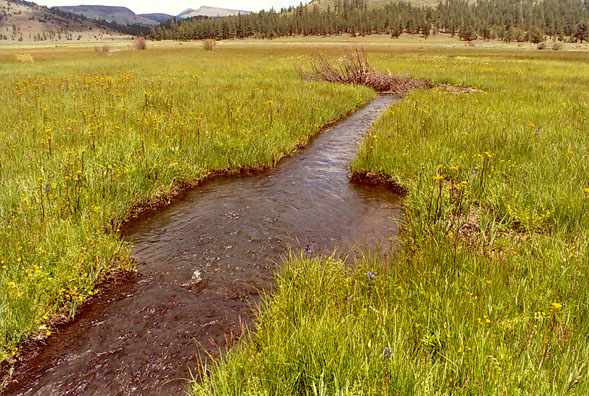
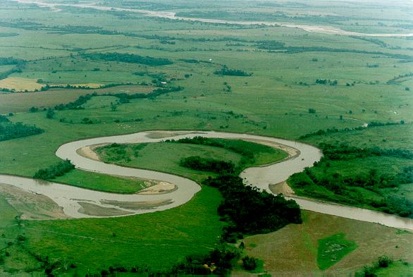
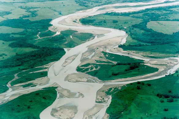
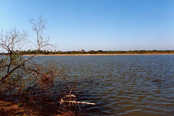
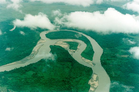
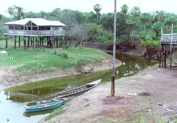
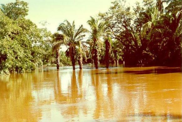
In general, there are two kinds of open channels: (1) natural, and (2) artificial. Natural channels are formed by Nature through geologic, geomorphologic, and hydrologic action. They include all natural watercourses, from the smallest to the largest. An example of a small watercourse is the small stream or rivulet shown in Fig. 2-1. An example of a large watercourse is the large river shown in Fig. 2-2. The largest natural channel is the Amazon river at its mouth, shown in Fig. 2-3. Applications of open-channel hydraulics in natural streams are typically in the fields of flood control, navigation, and stream restoration.
|
|
|
Artificial channels are also referred to as canals. They are made by humans for a specific purpose, usually to transfer water from a place where it exists in ample supply to a place where it is in short supply, or to transfer water between two locations to satisfy daily, monthly, seasonal, or annual requirements. Artificial channels are also built for flood control and navigation.
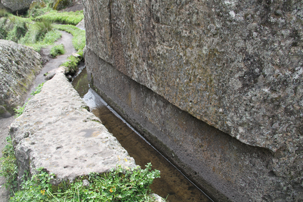
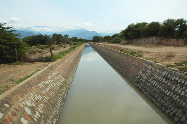
Artificial canals have been built by ancient societies, usually to transfer water for irrigation or water supply. For instance, Fig. 2-4 shows a small canal built about 3,500 years ago by the ancient people of Cajamarca, Peru.
|
Artificial channels can be referred to with various names, depending on their features and intended use:
-
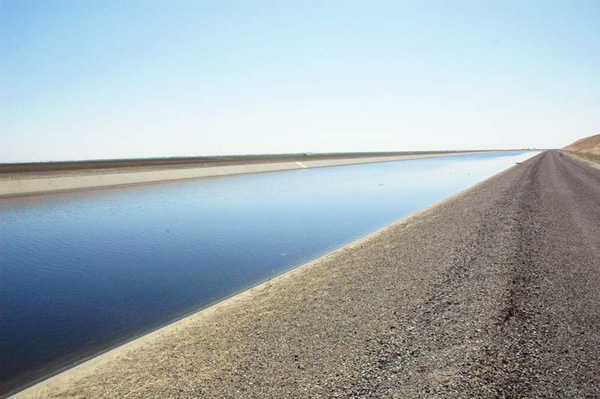
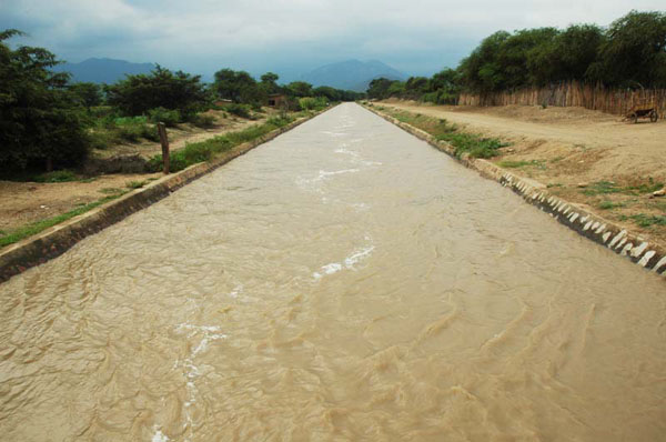
Canal: Usually long, generally of mild slope, lined or unlined, ground supported. The lining can be of various materials, such as concrete, masonry, asphalt, or wood (Fig. 2-5).
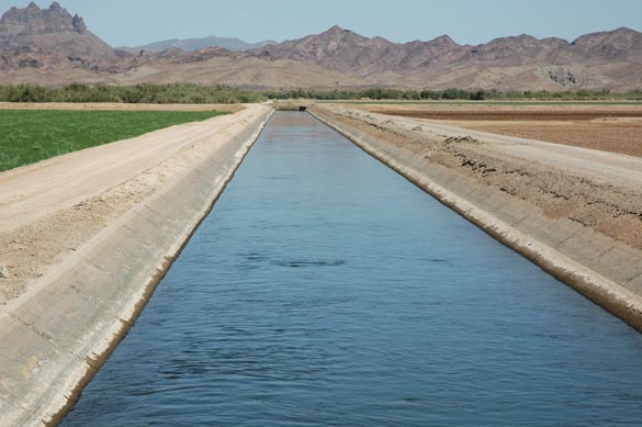
Fig. 2-5 Irrigation canal, Wellton-Mohawk Irrigation District, Wellton, Arizona.
-
Flume: An open-channel conduit, supported above ground, either full scale or laboratory scale. Llining can be of various materials, such as metal, wood, or acrylic plastic (Fig. 2-6).
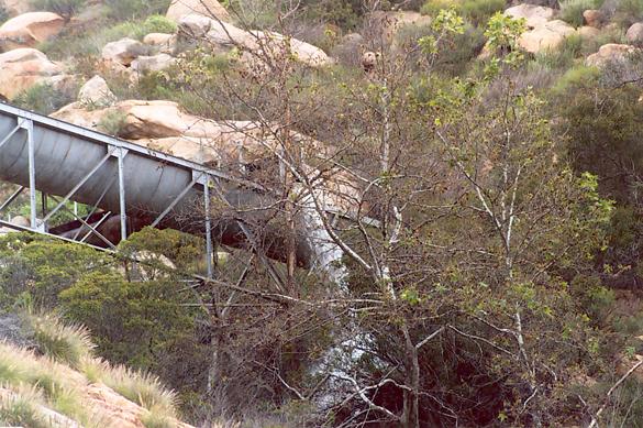
Fig. 2-6 The Dulzura conduit, in San Diego County, California,
overflowing after heavy rain, on March 5, 2005. -
Chute: A canal of very steep slope (Fig. 2-7).
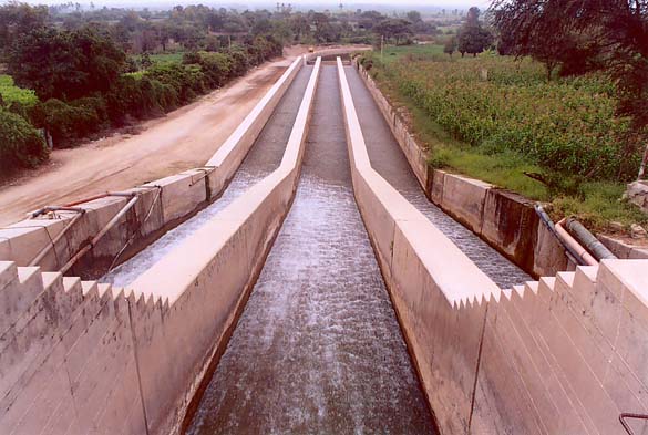
Fig. 2-7 Chute at Taymi Canal, Lambayeque, Peru.
-
Drop: A chute within a very short distance, usually to follow the topography (Fig. 2-8).
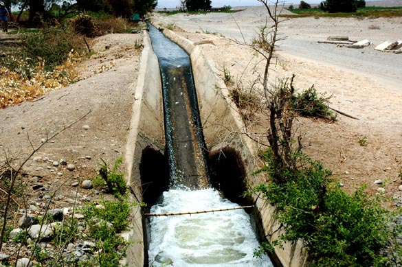
Fig. 2-8 Drop in an irrigation canal, Arequipa, Peru.
-
Aqueduct: A canal to transport water for a specific use, typically over terrain, or elevated over a valley, stream or road (Fig. 2-9).
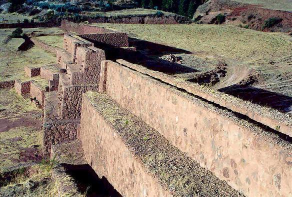
Fig. 2-9 Wari aqueduct at Sumaq Tika, Cuzco, Peru, dated c. 1000 A.D.
-
Culvert: A covered conduit (or conduits) of relatively short length, usually flowing partially full, to enable a stream to cross a highway or other embankment (Fig. 2-10).
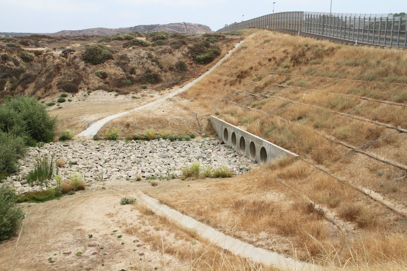
Fig. 2-10 Culvert crossing the U.S.-Mexico border at Yogurt Canyon, California.
Uses of Open Channels
Open channels, both natural and artificial, are used in various water resources fields, including:
- Irrigation and drainage,
- Flood control,
- Urban drainage,
- Hydropower generation,
- River navigation,
- Urban water supply,
- Wastewater disposal, and
- Stream restoration.
Figure 2-11 shows a fish-passage channel at a pond-and-plug stream restoration site in Ferris Creek, Plumas County, California.
|
Related Fields
Other related fields that benefit directly from open channel hydraulics knowledge include:
Hydrology: The study of water in the hydrologic cycle.
Fluvial geomorphology: The study of the genesis and shape of streams and rivers.
River mechanics: The study of the mechanical properties and behavior or rivers.
Fluvial sedimentology: The study of fluvial sediments, including their source, transport, and fate.
Hydroclimatology: The study of climate and the hydrologic cycle.
Ecohydrology: The study of the interaction between water and vegetation in the hydrologic cycle.
Potamology: The scientific study of rivers.
2.2 CHANNEL GEOMETRY
|
|
Natural channels refer to the great number of streams and rivers around the world. With respect to longitudinal orientation, natural channels are classified as: (a) straight, (b) meandering, or (c) braided.
A straight channel is one that follows more or less a straight path. Conversely, a meandering channel curves around in plan view, as shown in Fig. 2-12. The ratio of stream length to valley length is referred to as sinuosity. The sinuosity of the stream shown is about 5.
|
A braided channel features multiple interconnected meandering subchannels (Fig. 2-13). The flow and sediment conditions under which a channel assumes a certain longitudinal shape is a subject of fluvial geomorphology.
|
During floods, natural channels may overflow their banks and temporarily take up significant portions of the adjacent floodplain (Fig. 2-14). With respect to flood stage, flow in natural channels is classified as: (1) inbank, when the flow remains in the main channel, or (2) overbank, when the flow spills over to the adjacent floodplains.
|
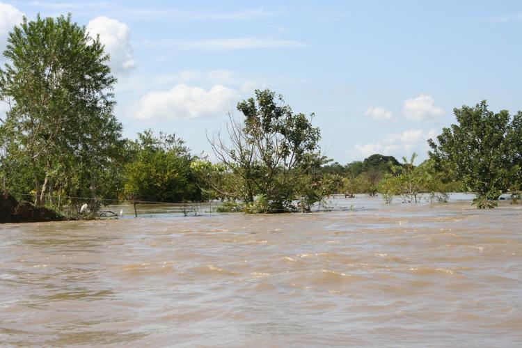
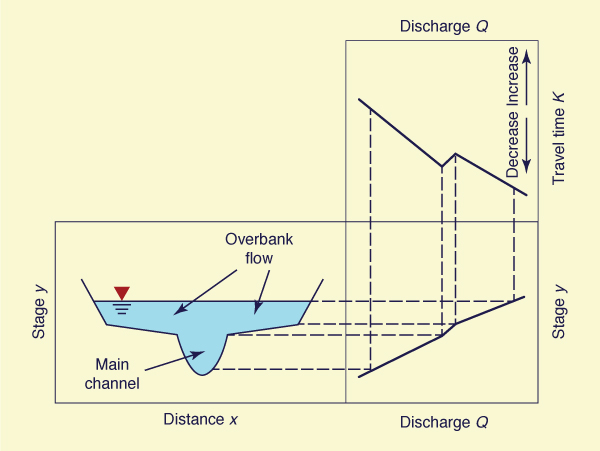
Figure 2-15 shows the typical variation of stage and flood wave travel time K with extent of inundation. These variations are due to relative increases or decreases of surface bottom friction as the stage increases.
|
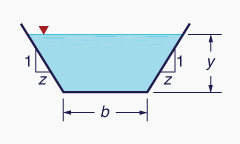
Artificial channels are classified as either: (1) prismatic, or (2) nonprismatic. Prismatic channels have a constant cross section, either trapezoidal, rectangular, or triangular. Trapezoidal channels are the most common type (Fig. 2-16). Rectangular channels are often used in sanitary flows and laboratory applications. Triangular channels are normally used in road and urban drainage.
|
Nonprismatic channels are those for which the cross section is not constant. Nonprismatic channels are used in the transition from a cross section of one size to another of a different size, usually to account for the variability in bottom slope.
Hydraulically wide channel
There are three asymptotic cross-sectional shapes in prismatic channels (Section 1.3):
- Hydraulically wide, for which the wetted perimeter is a constant,
- Triangular, for which the top width is proportional to the flow depth (Fig. 1-9), and
- Inherently stable, for which the hydraulic radius is a constant (Fig. 1-10).
A channel is hydraulically wide when the wetted perimeter P can be approximated by the top width T. By definition, the hydraulic radius R is equal to the flow area A divided by the wetted perimeter P. Likewise, the hydraulic depth D is equal to the flow area A divided by the top width T. Therefore, the following relations hold for a hydraulically wide channel:
|
P ≅ T | (2-1) |
|
R ≅ D | (2-2) |
In practice, a channel may be considered hydraulically wide if the top width T is greater than or equal to 10 times the hydraulic depth D (Chow, 1959):
|
T _____ ≥ 10 D | (2-3) |
In general:
|
Q = V A | (2-4) |
in which Q = discharge, A = flow area, and V = mean velocity. Since by definition:
|
A = D T | (2-5) |
it follows that:
|
Q = V D T | (2-6) |
and:
|
q = V D | (2-7) |
in which q = discharge per unit of channel width, or unit-width discharge [L2 T -1].
For simplicity, a hydraulically wide channel may be analyzed in terms of its unit-width discharge. For a hypothetical unit-width channel, the wetted perimeter is a constant: P = T = 1. Therefore, a hydraulically wide channel is alternatively defined as that for which the wetted perimeter is a constant. In practice, most natural channels are hydraulically wide (Fig. 2-17).
|
Hydraulics of the cross section
The discharge-flow area rating in open-channel flow is:
|
Q = α Aβ | (2-8) |
The asymptotic values of β are (Section 1.3):
β = 5/3 for a hydraulically wide channel with turbulent Manning friction,
β = 3/2 for a hydraulically wide channel with turbulent Chezy friction,
β = 4/3 for a triangular channel with turbulent Manning friction,
β = 5/2 for a triangular channel with turbulent Chezy friction, and
β = 1 for an inherently stable channel.
For trapezoidal channels, values of β lie between the
values for hydraulically wide and triangular channels. Typical values of
β for trapezoidal channels lie approximately
in the range
|
Depth of flow and depth-of-flow section
There are two related depths of open-channel flow (Fig. 2-19):
- The depth of flow y, and
The depth-of-flow section d.
The depth of flow y is the vertical distance from the free surface to the lowest point in the channel cross section. The depth-of-flow section d is the distance, normal to the direction of flow, measured from the free surface to the lowest point in the channel cross section.
|
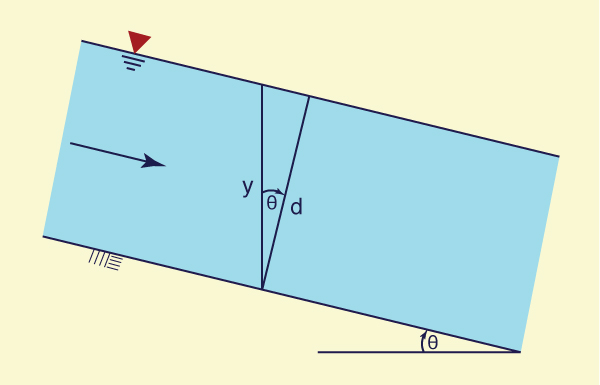
The relation between depth of flow y and depth of flow section d is:
|
d = y cos θ | (2-9) |
Geometric elements
Table 2-1 shows geometric elements for four commonly used cross-sectional shapes.
| Table 2-1 Geometric elements of four commonly used cross-sectional shapes. | |||||||||
| Shape (Click on figure to enlarge) |
Area A |
Wetted perimeter P |
Top width T |
Hydraulic radius R |
Hydraulic depth D |
||||
 |
by | b + 2y | b |
|
y | ||||
 |
|
|
|
||||||
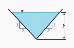 |
zy2 | 2zy |
|
y ___ |
|||||
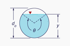 |
|
θ do ______ 2 |
|
|
|||||
2.3 VELOCITY DISTRIBUTION
|
|
The mean velocity in open-channel flow is:
|
Q V = _____ A | (2-10) |
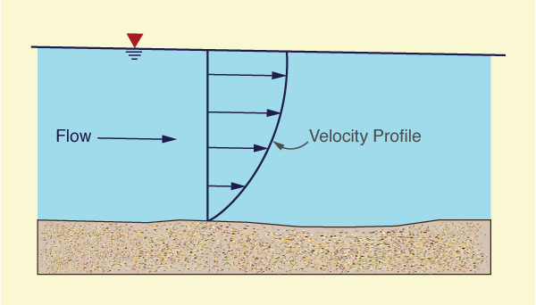
Local velocities, however, are likely to vary widely. Vertical velocity profiles vary from zero at the boundary (the no-slip condition at the channel bottom) to values slightly greater than the mean near the water surface (Fig. 2-20).
|
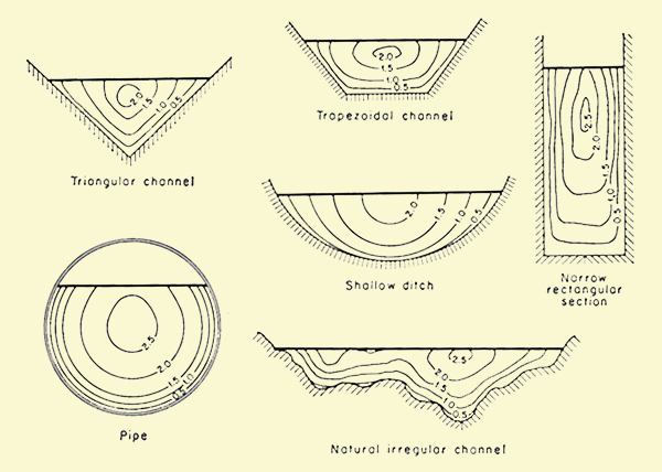
Transversal velocities are also likely to vary widely, from zero at the side boundaries to maximum values at or near the middle of the channel (Fig. 2-21). In meandering channels, or channels of curved alignment, velocities are larger along the outside of the bend and smaller on the inside. However, for hydraulically wide channels, the sides have a negligible influence on the flow. In this case, the flow is effectively two-dimensional (in the longitudinal and vertical directions).
|
The assumption of mean velocity V (Eq. 2-10) further reduces the flow to a statement of one-dimensionality (in the longitudinal direction). This assumption is strictly applicable to channels that are relatively straight and for which flows remain inbank. As a convenient approximation, the one-dimensional assumption has been applied to channels with mild meandering tendencies and limited overbank flows. However, the one-dimensional assumption generally breaks down for channels of large sinuosity and/or substantial overbank flows (Fig. 2-22).
|
2.4 MEASUREMENTS OF VELOCITY
|
|
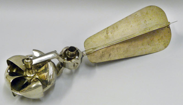
Measurements of velocity are commonly performed using a current meter. Current meters measure flow velocity by counting the number of revolutions per second of the meter assembly. The rotation can be around a vertical axis, leading to the cup meter, or around a horizontal axis, leading to the propeller meter.
Cup meters are widely used in the United States. The most common type of cup meter is the Price current meter, which has six cups mounted on a vertical axis (Fig. 2-23). The flow velocity is proportional to the angular velocity of the meter rotor. The flow velocity is determined by counting the number of revolutions per second of the rotor and consulting the meter calibration table.
|
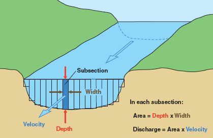
Discharge measurements. A discharge measurement at a stream cross section requires the determination of flow area and mean velocity for a given stage. The cross section should be perpendicular to the flow, and mean velocity should be based on a sufficient number of velocity measurements across the section.
In a typical stream-gaging procedure, each of several depth soundings, usually 20 to 30, defines the position of a vertical (Fig. 2-24). Each depth sounding is associated with a partial section of the stream. A partial section is a rectangle of depth equal to the sounding and of width equal to half the difference of the distances to adjacent verticals. At each vertical, the following observations are made:
- The flow depth, and
- The velocity as measured by a current meter at one or two points along the vertical.
|
In the two-point method, the current meter is positioned at 0.2 and 0.8 of the flow depth. In the one point method, the current meter is positioned at 0.6 of the flow depth, measured from the water surface. The average of the velocities at 0.2 and 0.8 depth or the single velocity at 0.6 depth is taken as the mean velocity in the vertical. Where a two-point measurement is impractical (e.g., in very shallow streams), the one-point method is recommended.
For each partial section, the discharge is calculated as:
| q = v a | (2-11) |
in which q = discharge, v = mean velocity, and a = flow area. The total stream discharge Q is the sum of the discharges of each partial section.
Price current meters types AA and A are used for two-point velocity measurements in streams with flow depths above 0.75 m and for one-point measurements in streams with depths ranging from 0.45 to 0.75 m. The dwarf (or pigmy) current meter is used for one-point measurements in shallow streams or laboratory flumes with depths in the range 0.10 to 0.45 m.
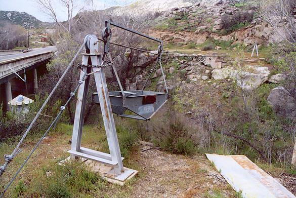
Techniques for measuring stream velocity with a current meter vary with stream size. If the stream is wadable, the meter is affixed to a graduated depth rod. If the stream is too deep to wade, the meter is suspended on a cable and is held in the water with a sounding weight. The weights are made of various sizes, from 6.8 kg to 135 kg. Measurements using cable suspension are made from bridges, cableways, or boats (Fig. 2-25). For the heavier sounding weights or when using a boat, a sounding reel may be required.
|
2.5 VELOCITY DISTRIBUTION COEFFICIENTS
|
|
Due to the nonuniform velocity distribution over a cross section, the true velocity head hv is greater than the velocity head computed based on the mean velocity V. Generally, the true velocity head is:
|
V 2 hv = α ____ 2g | (2-12) |
where in this case α refers to the energy coefficient, or Coriolis coefficient. Values of α range from about 1.03 to 1.36 for fairly straight prismatic channels. The higher values correspond to smaller channels and the lower values to larger channels.
Similarly to the case of energy, momentum also requires a correction due to the nonuniform velocities (Fig. 2-26). The true expression for momentum flux (force) is:
|
F = β ρ Q V | (2-13) |
where in this case β refers to the momentum coefficient, or Boussinesq coefficient; and ρ = mass density of water. Values of β range from about 1.01 to 1.12 for fairly straight prismatic channels.
Values of α and β are slightly greater than 1, with α being always greater than β.
For channels of composite cross section, values of α and β can easily get as great as
1.6 and 1.2, respectively
|
The Coriolis coefficient
Assume:
- A = total area of the cross section ... [L2]
- V = mean velocity of the cross section ... [L T -1]
- ΔA = incremental area ... [L2]
- v = velocity through incremental area ΔA ... [L T -1]
The mean velocity is defined as:
|
Σ
v ΔA V = ____________ ... [L T -1] Σ ΔA | (2-14) |
In general, energy is equal to a force integrated over a distance, or force times length:
|
E = ∫ F ds = F L ... [F L] | (2-15) |
The kinetic energy for the total area A is equal to mass M times acceleration times distance:
|
1 E = ____ M V 2 ... [M L 2 T -2] 2 | (2-16) |
The kinetic energy for the incremental area ΔA is:
|
1 ΔE = ____ m v 2 ... [M L 2 T -2] 2 | (2-17) |
The velocity head through ΔA is the kinetic energy divided by the weight, where weight = mg :
|
v 2 hv = ______ ... [L] 2 g | (2-18) |
The volumetric flux through ΔA is:
|
ΔQ = v ΔA ... [L 3 T -1] | (2-19) |
The weight flux through ΔA is:
|
Δ(WF) = γ v ΔA ... [F T -1] | (2-20) |
in which γ = unit weight of water.
The incremental kinetic energy flux through ΔA
is equal to the kinetic energy per weight hv
|
γ v 3 ΔA Δ(EF) = ___________ ... [F L T -1] 2 g | (2-21) |
The sum of kinetic energy fluxes for all incremental areas is:
|
γ v 3 ΔA ∑ Δ(EF) = ∑ ___________ ... [F L T -1] 2 g | (2-22) |
The kinetic energy flux through the total area A, based on mean velocity V, is:
|
γ V 3 A (EF) = α ___________ ... [F L T -1] 2 g | (2-23) |
Equating Eqs. 2-22 and 2-23, and solving for the Coriolis energy coefficient:
|
Σ v 3 ΔA α = _____________ V 3 A | (2-24) |
The Boussinesq coefficient
The mass flux
J through the total area A is equal to the mass density ρ times the
volumetric flux
|
J = ρ V A ... [M T -1] | (2-25) |
The mass flux through the incremental area ΔA is equal to the mass density ρ times the incremental volumetric flux ΔQ = v ΔA:
|
ΔJ = ρ v ΔA ... [M T -1] | (2-26) |
In general, momentum M is equal to a force integrated over a period of time, or mass times velocity:
|
M = ∫ F dt = m V ... [M L T -1 ] | (2-27) |
The momentum flux, or force F, is equal to the mass flux times the velocity. Thus, the momentum flux through the incremental area ΔA is:
|
ΔF = ρ v 2 ΔA ... [F = M L T -2] | (2-28) |
The sum of all momentum fluxes, or sum of forces for all the incremental areas is:
|
∑ ΔF = ∑ ρ v 2 ΔA ... [F] | (2-29) |
The momentum flux, or force F, through the total area is:
|
F = β ρ V 2 A ... [F] | (2-30) |
Equating Eqs. 2-29 and 2-30, and solving for the Boussinesq momentum coefficient:
|
Σ v 2 ΔA β = _____________ V 2 A | (2-31) |
|
Approximate formulations of α and β
While Eqs. 2-24 and 2-31 are accurate, they require detailed measurement of the velocity distribution in the cross section of interest. Alternatively, when only the mean velocity V and maximum velocity Vmax are known, the following formulas may be used to calculate approximate values of the Coriolis and Boussinesq coefficients (Chow, 1959). Defining:
|
Vmax ε = ________ - 1 V | (2-32) |
Assuming a logarithmic velocity distribution, the coefficients may be approximated as:
|
α = 1 + 3ε 2 - 2ε 3 | (2-33) |
|
β = 1 + ε 2 | (2-34) |
On the other hand, assuming a linear velocity distribution:
|
α = 1 + ε 2 | (2-35) |
|
ε 2 β = 1 + _____ 3 | (2-36) |
2.6 PRESSURE DISTRIBUTION
|
|
The pressure distribution along the flow depth in an open channel varies with the shape of the channel bottom relative to the shape of the water surface, measured along the direction of flow. There are three possible cases: (1) parallel flow, (2) convex curvilinear flow, and (3) concave curvilinear flow.
Parallel flow
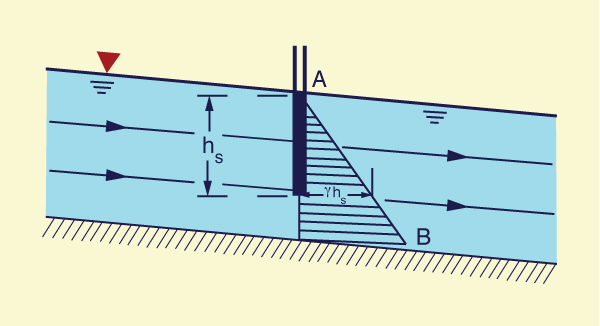
Under parallel flow, the channel bottom is relatively straight and it is either: (a) parallel to the water surface, as with uniform flow (Fig. 2-28), or (b) approximately parallel to the water surface, as with gradually varied flow. In this case, the pressure distribution is essentially hydrostatic, with the pressure varying as a linear function of partial flow depth (line AB in Fig. 2-28). At the partial flow depth hs, the pressure is: ps = γ hs. In other words, a piezometer located at the partial depth hs below the water surface would rise to the elevation of the water surface.
|
In practice, uniform flow
and gradually varied flow feature a hydrostatic pressure distribution
|
Convex curvilinear flow
Under convex curvilinear flow,
the channel
bottom is substantially curved,
featuring a convex profile in the vertical plane (Fig. 2-30).
In this case,
the pressure distribution is nonhydrostatic, with the pressure along the flow depth
varying as a nonlinear function of
partial flow depth (curve AB' in
|
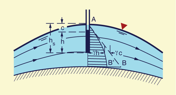
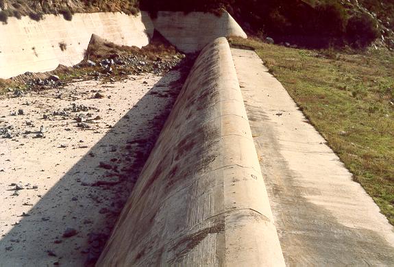
In practice, rapidly varied flow, e.g., flow over the crest of an ogee spillway, features a nonhydrostatic pressure distribution (Fig. 2-31). This distribution is characterized by substantial velocity components and accelerations in the direction normal to the flow.
|
Concave curvilinear flow
Under concave curvilinear flow,
the channel
bottom is substantially curved, featuring a concave profile in the vertical plane (Fig. 2-32).
In this case,
the pressure distribution is nonhydrostatic, with the pressure along the flow depth
varying as a nonlinear function of partial flow depth (curve AB'
in
|
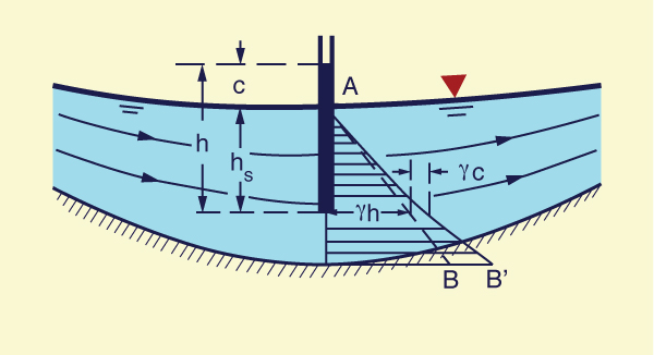
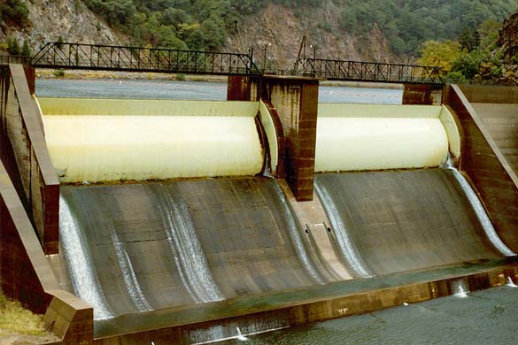
In practice, rapidly varied flow, e.g., flow at or near the toe of a spillway, features a nonhydrostatic pressure distribution (Fig. 2-33). This distribution is characterized by substantial velocity components and accelerations in the direction normal to the flow.
|
The centrifugal pressure head c can be approximately calculated as follows:
The centrifugal force is equal to the mass times the centrifugal acceleration (f = m × a).
The centrifugal pressure pc is equal to the mass per unit of area times the centrifugal acceleration.
The centrifugal pressure head c is equal to the centrifugal pressure divided by the unit weight of water (γ).
The mass per unit of area is:
|
Mass/Area = ρ (Volume/Area) = ρ d = (γ/g) d ... [M L -2 = F T 2 L -3] | (2-37) |
in which d = flow depth.
The centrifugal acceleration is:
|
V 2 a = ______ ... [L T -2] r | (2-38) |
in which r = radius of curvature of the streamlines.
Thus, the centrifugal pressure is Eq. 2-37 times Eq. 2-38:
|
γd V 2 pc = _____ _____ ... [F L -2] g r | (2-39) |
and the centrifugal pressure head is:
|
d V 2 c = ____ _____ ... [L] g r | (2-40) |
The rise is negative for convex curvilinear flow and positive for concave curvilinear flow (Fig. 2-34).
|
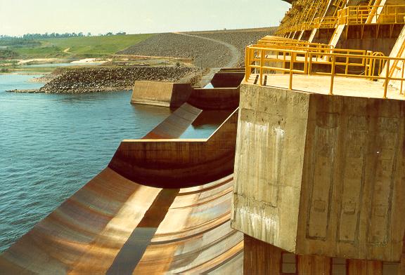
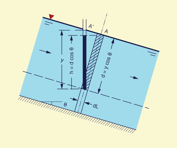
Effect of slope on pressure distribution
Figure 2-35 shows a schematic of the pressure distribution in a channel of steep slope θ. Note the following:
The weight of the shaded element is: γ d [dL (1)] = γ y cosθ [dL (1)]
The pressure exerted by the shaded element is: γ h = γ d cosθ = γ y cos2θ
The pressure rise is:
h = d cos θ = y cos2θ ... [L]
(2-41)
For a channel of small slope, h ≅ y, and the vertical depth y may be used to estimate the pressure rise h. However, for a channel of large slope, the difference may be substantial.
A 10% slope (i.e., a slope equal to 0.1) corresponds to an angle θ = 5.7°, for which cos2 (5.7°) = 0.99. Thus, for a slope greater than 10%, the error in taking the vertical depth y in lieu of the pressure rise h is more than 1%. A channel with slope greater than 10% is referred to as a channel of large slope.
|
In practice, a channel of large slope features high velocities, which may lead to air entrainment, volume swell, and consequent increase in depth and decrease in density. Thus, the pressure calculated by Eq. 2-41 may be somewhat higher that the actual value.
QUESTIONS
|
|
What is a chute?
What is an aqueduct?
What is a culvert?
What is potamology?
What is sinuosity in connection with rivers?
What is a hydraulically wide channel?
What ratio of top width to hydraulic depth can be considered hydraulically wide?
What is the typical range of the exponent β for trapezoidal channels?
What is the most common type of current meter in the United States?
Why is the true velocity head greater than the velocity head computed based on mean velocity?
How does energy differ from momentum?
How does the pressure distribution in the vertical vary under parallel flow?
How does the pressure distribution in the vertical vary under convex curvilinear flow?
How does the pressure distribution in the vertical vary under concave curvilinear flow?
What is a channel of large slope?
PROBLEMS
|
|
What is the discharge per unit of width if the discharge is 24 m3/s and the channel top width is
T = 8 m? Given: coefficient of the rating α = 0.4; exponent β = 1.55; flow area A = 45.6 m2. What is the discharge Q?
Given culvert diameter do = 1 m; what is the flow area for θ = 300°? (See Table 2-1).
What is the force F developed by a discharge Q = 10 ft3/s at a velocity V = 1 ft/s, at a cross section with a Boussinesq coefficient β = 1.05?
A stream of flow area A = 100 m2 is divided into three sections: (1) left overbank, with 20% of the flow area, and velocity
0.2 m/s; (2) inbank center, with 70% of the flow area, and velocity1 m/s; and (3) right overbank, with 10% of the flow area, and velocity0.1 m/s. Calculate the Coriolis coefficient α and the Boussinesq coefficient β.
Fig. 2-36 A composite cross section.
Calculate the velocity distribution coefficients for the following canal data, with flow area
A = 2768 ft2. Increment Velocity v
(ft/s)Incremental
flow area ΔA (%)1 3.5 0.5 2 4.0 2.9 3 4.5 10.3 4 5.0 23.5 5 5.5 52.7 6 6.0 10.1 Compare the results with those of approximate logarithmic formulas.
A spillway is designed for a discharge q = 5 m2/s with a flow depth d = 0.5 m. What is the minimum radius of curvature of the spillway cross section to ensure that the pressure does not fall below 50% of hydrostatic?
REFERENCES
|
|
Chow, V. T. 1959. Open-channel Hydraulics. McGraw Hill, New York.
Ponce, V. M., and D. Windingland. 1985. Kinematic shock: Sensitivity analysis. Journal of Hydraulic Engineering, ASCE, Vol. 111, No. 4, April, 600-611.
| http://openchannelhydraulics.sdsu.edu |
|
140906 21:00 |