|
|
|
CHAPTER 11: SUBSURFACE WATER |
|
"In my experience, the recharge, and certainly the change in recharge due to a development (induced recharge), is difficult, if not impossible, to quantify." John Bredehoeft (1997) |
|
This chapter is divided into five sections. Section 11.1 describes general properties of subsurface water; Section 11.2 describes physical properties; Section 11.3 describes the equations of groundwater flow; Section 11.4 deals with well hydraulics; and Section 11.5 discusses surface-subsurface flow interaction, including concepts of hillslope hydrology, streamflow generation, and baseflow recession. |
11.1 GENERAL PROPERTIES OF SUBSURFACE WATER
|
|
The study of surface water is incomplete without the knowledge of its interaction with subsurface water. Subsurface water comprises all water either in storage or flowing below the ground surface. There are two types of subsurface water: (1) interflow, and (2) groundwater flow. Interflow takes place in the unsaturated zone, close to the ground surface. Groundwater flow takes place in the saturated zone, which may be either close to the ground surface or deep in underground waterbearing formations. The surface separating the unsaturated and saturated zones is referred to as the groundwater table, or water table.
In Section 2.4, the following three components of runoff were identified: (1) surface runoff, (2) runoff contributed by interflow, and (3) runoff contributed by groundwater, i.e., baseflow. These components depict the path of runoff. At any one time, runoff consists of a combination of the three. Generally, during wet-weather periods, surface runoff and interflow are the primary contributors to runoff. Conversely, during dry-weather periods, baseflow is the major--if not the only--contributor to runoff.
Traditionally, surface runoff has been regarded as the single most important component of flood flows. This approach is embodied in the concept of overland flow, or Hortonian flow, after Horton, who pioneered the theory of infiltration capacity [12]. As shown in Chapters 4 and 10, overland flow can be used to simulate runoff response.
Notwithstanding the classical Hortonian approach, theories of hillslope hydrology have emphasized the role of interflow and the timing--rather than the path--of runoff. Two runoff components are recognized under this framework:
Quickflow, consisting of overland flow, fast interflow, and rain falling directly on the channel network, and
Baseflow, consisting of slow interflow and groundwater flow [11].
Subsurface water occurs by infiltration of rainfall and/or snowmelt into the ground. Once the water has infiltrated, it can follow one of two paths:
Move in a general lateral direction within the unsaturated zone close to the ground surface, or
Move in a general downward direction and join the saturated zone.
The preferred path of subsurface flow is in a downward direction to join the saturated zone. Interflow is flow in the unsaturated zone; groundwater flow is flow in the saturated zone.
The earth's crust is composed of soils and rocks containing pores (i.e., voids) that can hold air and water. The various types of soils and rocks have different relative amounts of pore space and, consequently, can hold different amounts of air and water. In subsurface water evaluations, the earth's crust is divided into two zones:
-
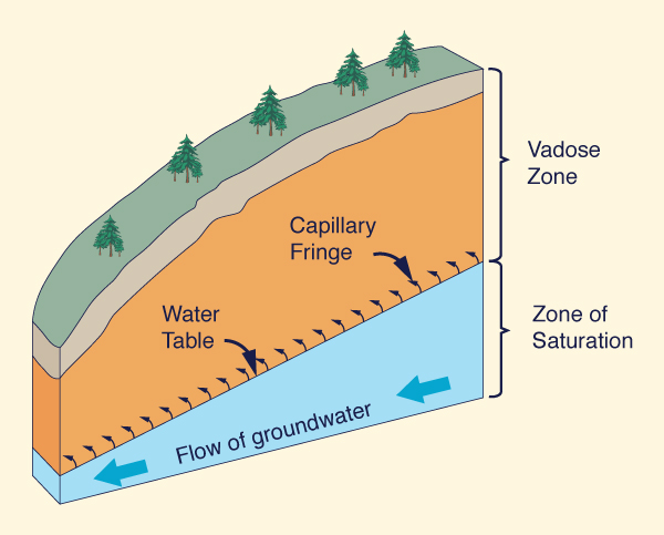
The unsaturated zone, or vadose zone, where the pores are filled with both air and water, and
The saturated zone, or zone of saturation, where the pores are filled only with water.
The boundary between the unsaturated and saturated zones is the water table.
Figure 11-1 The vadose zone and the zone of saturation. |
The distance from the ground surface to the water table varies from place to place. In some places it may be less than 1 m, whereas in others it may be more than 100 m. In general, the water table is not flat, tending to follow the surface topography in a subdued way, deeper beneath the hills and shallower beneath the valleys. In certain cases it may even coincide with the ground surface, as with ponds and marshes, or lie slightly above it, as in the typical exfiltration to perennial streams and rivers.
Extent of Groundwater Resources
Although only a fraction of precipitation infiltrates into the ground, the total amount of subsurface water is far greater than the total amount of land surface water. This is because groundwater flow is characteristically a very slow process, whereas land surface water moves at comparatively faster speeds. The average residence time of surface water (i.e., the time elapsed while flowing on the earth's surface) is estimated at less than 2 wk. On the other hand, the average residence time of subsurface water has been estimated to vary between 2 wk to 10,000 yr [19] . Both surface and subsurface water are driven by the force of gravity in their unrelenting movement toward the sea.
To place the relationship between surface and subsurface water amounts in the proper perspective, it is necessary to examine the world's water balance. Studies have shown that about 97 percent of all the world's water is seawater. Of the remaining 3 percent, one-third occurs in solid form in glaciers and polar ice caps, and two-thirds constitutes fresh water, including surface and subsurface water. Of the total amount of fresh water, more than 99 percent is groundwater. The water stored in lakes, reservoirs, streams, rivers, the unsaturated zone below the ground surface, and in vapor form in the atmosphere accounts for only a small fraction of the total amount of fresh water [8].
About half of the groundwater is contained within 800 m of the earth's surface [20]. Not all can be used, either because of its salinity or because of the great depths at which it occurs. The distribution of groundwater varies throughout the land areas of the world. Where it does occur, it can been used to supplement surface water supplies. Furthermore, in regions with little or no surface water resources, groundwater is often the only source of fresh water.
|
A note of caution is necessary here. While groundwater quantities exceed surface water quantities by at least two orders of magnitude, surface water has the advantage that is is fully recyclable in the short term (with a global average of every 11 days), while groundwater is not [18]. Thus, depletion of groundwater (sometimes referred to as "overdraft") effectively amounts to mining, since the time required for replenishment would be too long for practical consideration (hundreds to thousands of years). Furthermore, where surface and groundwater systems are interconnected, groundwater overdraft generally leads to loss of baseflow and the progressive aridization of the landscape. |
The feasibility of extracting water from a groundwater reservoir is determined by the following three properties: (1) porosity, (2) permeability, and (3) replenishment. Porosity is the ratio of void volume to total volume of soil or rock. It is interpreted as a measure of the ability of the soil deposit or rock formation to hold water in sufficiently large quantities.
Permeability describes the rate at which water can pass through a soil deposit or rock formation. Permeable materials are those that allow water to pass through them easily. Conversely, impermeable materials are those that allow water to pass through them only with difficulty or not at all. The permeability value is a function of the size of pores or voids and the degree to which they are interconnected.
Replenishment relates to the size and extent of the groundwater reservoir and its connection to other surface/groundwater resources of the region. Replenishment is largely controlled by nature, although it can be affected by human activities, both positively (e.g., the artificial recharge of groundwater), and negatively (by paving formerly porous land).
Aquifers
An aquifer is a saturated permeable geologic formation which can yield significant quantities of water to wells and springs. By contrast, an aquiclude is a saturated geologic formation that is incapable of transmitting significant amounts of water under ordinary circumstances.
The term aquitard describes the less permeable beds in a stratigraphic sequence. These beds may be permeable enough to transmit water in significant quantities, but not sufficient to justify the cost of drilling wells to exploit the groundwater resource. Most geologic formations are classified as either aquifers or aquitards, with very few formations fitting the definition of an aquiclude.
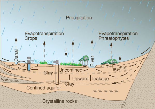
Aquifer Types. Aquifers can be of two types: (1) unconfined and (2) confined. An unconfined aquifer, or water table aquifer, is an aquifer in which the water table constitutes its upper boundary. A confined aquifer is an aquifer that is confined between two relatively impermeable layers or aquitards. Unconfined aquifers occur near the ground surface; confined aquifers occur at substantial depths below the ground surface. Figure 11-2 shows typical configurations of confined and unconfined aquifers.
The water level in an unconfined aquifer rests at the water table. In a confined aquifer, the water level in a well may rise above the top of the aquifer. If this is the case, the well is referred to as an artesian well, and the aquifer is said to exist under artesian conditions. In some cases, the water level may flow above the ground surface, in which case the aquifer is known as flowing artesian well, and the aquifer is said to exist under flowing artesian conditions.
Figure 11-2 (a) Groundwater flow through an unconfined acquifer [26]. |
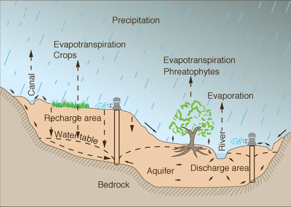
Figure 11-2 (b) Groundwater flow through an unconfined acquifer, a confined aquifer, |
The water level in wells located in a confined aquifer defines an imaginary surface referred to as the potentiometric surface [8]. Several wells can help establish a potentiometric contour map, a map depicting lines of equal hydraulic head in the aquifer. A potentiometric map provides an indication of the direction of groundwater flow in an aquifer.
A perched aquifer is a special case of unconfined aquifer. A perched aquifer forms on top of an impermeable layer located well above the water table. Infiltrating water is held on top of this impermeable layer to form a saturated lens, usually of limited extent and not connected to the main water table. The water table of a perched aquifer is referred to as a perched water table.
Recharge and Discharge. Typically, groundwater flows from a recharge area, through a groundwater reservoir, to a discharge area. The recharge area is an area of replenishment with infiltrated water. The groundwater reservoir is the main body of the aquifer. The discharge area is the area where the infiltrated water returns back to the surface. Most of the groundwater eventually returns to the surface before reaching the oceans [31].
In humid and subhumid climates, aquifer recharge usually takes place in upland slopes, with aquifer discharge occurring in the valleys, where the water table is shallow enough to be intercepted by streams and rivers. In arid and semiarid regions, however, the situation may be quite different. In this case, the water table in the valleys is usually much deeper, with aquifer recharge taking place primarily by channel transmission losses in streams and rivers.
Discharge from an unconfined aquifer is accomplished in three ways. First, if the water table is close to the ground surface, water may be discharged from the aquifer either by vapor diffusion upward through the soil or through evapotranspiration by vegetation. Second, if the water table is intersected by a stream, discharge is accomplished by exfiltration. Third, an aquifer can be discharged by human-induced means, i.e, by pumping through a well, either for agricultural, municipal, or industrial uses.
Discharge from a confined aquifer is accomplished in two ways: first, by fast seepage through a permeable path in the overlying impermeable material, or by slow seepage through aquitards; and second, by human-induced means, i.e., by well pumping as with unconfined aquifers [27].
11.2 PHYSICAL PROPERTIES OF SUBSURFACE WATER
|
|
In an unconfined aquifer, the water table is the surface at which the water pressure is exactly equal to atmospheric pressure. The soil or rock below the water table is generally considered to be saturated with water. Indeed, the water table is the upper limit of a zone of saturation, or saturated zone.
The capillary fringe is located immediately above the water table. Water is held in this fringe by capillarity, at moisture levels close to saturation. However, the capillary fringe differs from the saturated zone in that a well will fill with water only to the base of the capillary fringe, i.e., the water table. Water in the capillary fringe is referred to as capillary water to distinguish it from the water in the saturated zone, or groundwater proper.
The thickness of the capillary fringe varies from one rock formation to another, depending on the size of the pores, from a few millimeters to several meters. Due to natural irregularities, the top of the capillary fringe is likely to be an irregular surface, with the moisture likely to decrease gradually in a direction away from the water table.
Lowering of the water table by drainage, pumping, or other means will result in a lowering of the capillary fringe. However, all water cannot be drained out of the soil or rock formation. Surface tension and molecular effects are responsible for a certain amount of water being retained in the pores against the action of gravity.
Specific Yield
The total amount of water in an aquifer of area A and thickness b is
| V = A b n | (11-1) |
in which V = total volume of water, A = surface area of the aquifer, b = aquifer thickness, and n = porosity. However, the total amount of water that will drain freely from an aquifer is
| Vw = A b Sy | (11-2) |
in which Vw = volume of free-draining water and Sy = specific yield, the ratio of free-draining water volume to aquifer volume. Since a certain amount of water is always retained in the pore volume, the specific yield of an aquifer is always less than its porosity.
Specific retention is the ratio of volume of retained water to volume of aquifer. Therefore, the sum of specific yield and specific retention is equal to the porosity. In coarse-grained rocks with large pores, specific yield will be almost equal to the porosity, with specific retention reduced to a minimum. Conversely, in fine-grained rocks, specific retention can approximate the value of porosity, with specific yield being close to zero.
Above the capillary fringe is the intermediate zone, which may range in thickness from zero to more than 100 m. The water within this zone is referred to as pellicular water, with the water content generally close to specific retention. Above the intermediate zone is the upper portion of the earth's crust, referred to as the soil. The capillary fringe, the intermediate zone, and the soil are all part of the unsaturated zone. Interflow takes place in the unsaturated zone.
Soil Moisture Levels
Water enters the unsaturated zone by infiltration, where it is held in thin films around the solid particles or in the pore space between them. Within a given volume, the degree of saturation is a function of the relative amount of pore space that is occupied by water. The degree of saturation is a measure of the prevailing soil-moisture condition.
Field Capacity. Assume that a heavy rainfall causes significant amounts of water to infiltrate into the ground. If this situation persists for a sufficiently long period, the voids will eventually fill with water, i.e., a saturated condition will be attained.
During and immediately following rainfall, water will drain freely out of the soil under the effect of gravity, a characteristically slow process that can last anywhere from a few hours to several days. The total amount of water drained in this way represents the specific yield, with the remaining water constituting the specific retention. The moisture level equivalent to specific retention is the field capacity, i.e., the amount of water that can be held in the soil against the action of gravity.
Following a rainy period, evaporation from soil surfaces and evapotranspiration from vegetation act together to reduce the soil moisture below field capacity, and a soil-moisture deficit is gradually developed. The soil-moisture deficit is usually expressed in terms of the rainfall depth necessary to restore the soil moisture to field capacity.
Permanent Wilting Point. At or near field capacity, the water is largely held in thin films around the solid particles, with substantial amounts of air space between them. At the air-water interface, the difference in pressures (atmospheric in the air spaces and less than atmospheric within the thin films) results in a net suction effect. This suction effect, referred to as soil-water suction, keeps the water films adhered to the soil particles against the action of gravity.
With continuing absence of rainfall, increasing amounts of soil water are abstracted by evaporation, evapotranspiration, and vapor diffusion. This causes the water films surrounding the solid particles to become thinner and the soil-water suction to increase. Consequently, it becomes increasingly difficult for plants to extract water from the soil. Faced with this condition, the plants respond by using less water and reducing their growth rate. Plants that are deprived of normal amounts of water for an extended period of time begin to wilt. If water does not become available within a reasonable period, the permanent wilting point is reached and the plants die.
Flow Through Porous Media
The soil or rock deposits through which water flows can be regarded as porous media. The fundamental law governing flow through porous media is Darcy's law.
Darcy's Law. In 1856, Darcy pioneered the analysis of flow of water through sands [6]. His experiments led to the formulation of the empirical equation of flow through porous media bearing his name.
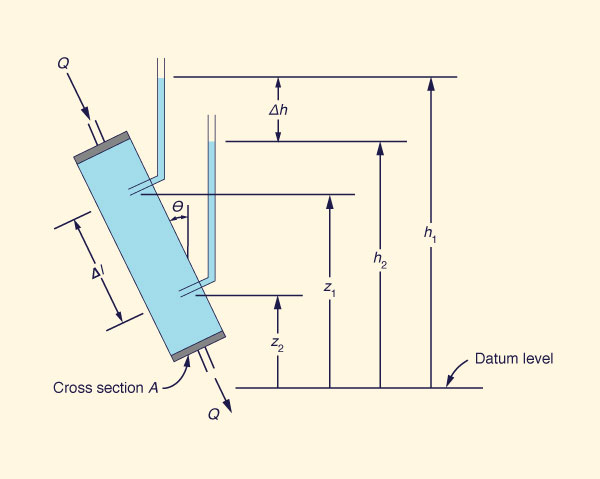
With reference to Fig. 11-3, Darcy's law states that the flow rate Q is directly proportional to the cross-sectional flow area A and hydraulic drop Δh and inversely proportional to the length Δl:
|
Δh Q = K A _____ Δl | (11-3) |
in which K is a proportionality constant known as the hydraulic conductivity. The quantity Δh/Δl is a dimensionless ratio referred to as hydraulic gradient i:
Figure 11-3 Experimental setup for the illustration of Darcy's law [8]. |
|
Δh i = _____ Δl | (11-4) |
Therefore,
| Q = K i A | (11-5) |
and
|
Q v = ___ = K i A | (11-6) |
is the specific discharge or discharge per unit area, with the dimensions of velocity. The specific discharge, also known as Darcy velocity or Darcy flux, is a macroscopic concept that can be readily measured. It must be clearly differentiated from the microscopic velocities associated with the actual paths of the water as it winds its way through porous media. These velocities are real but--for all practical purposes--intractable.
Darcy's law is valid for groundwater flow in any direction. Given a constant hydraulic conductivity and hydraulic gradient, the specific discharge is independent of the angle θ shown in Fig. 11-3. This holds even for values of θ greater than 90°, when the flow is being forced up through the cylinder against gravity.
Hydraulic Conductivity. The hydraulic conductivity, which according to Eq. 11-6 has the dimensions of velocity [LT -1], is a function of the physical properties of fluid and porous media. To illustrate, consider the experimental setup of Fig. 11-3. Assume two experiments, each consisting of two tests, with Δh and Δl being held constant. In the first experiment, the fluid is the same (e.g., water), and two types of porous media are tested: (1) a coarse sand and (2) a fine sand. The specific discharge of the second test (fine sand) will be smaller than that of the first test (coarse sand). In the second experiment, the porous medium is the same (e.g., coarse sand), and two fluids of different viscosity are tested: (1) water and (2) oil. The specific discharge of the second test (oil) will be smaller than that of the first test (water).
An expression for hydraulic conductivity in terms of fluid and porous media properties is [13]:
|
C d 2ρ g K = __________ μ | (11-7) |
in which d = mean grain diameter, ρ = fluid density, μ = fluid absolute viscosity, g = gravitational acceleration, and C = a dimensionless constant, a function of porous media properties other than mean grain diameter, i.e., grain size distribution, sphericity and roundness of the particles, and the nature of their packing.
Intrinsic Permeability. In Eq. 11-7, the product Cd 2 is a function only of the porous media, whereas ρ and μ are functions of the fluid. Therefore,
| k = C d 2 | (11-8) |
in which k is the specific, or intrinsic, permeability. From Eqs. 11-7 and 11-8,
|
k ρ g K = _______ μ | (11-9) |
Intrinsic permeability is expressed in square centimeters or, alternatively, in darcys. One darcy unit is defined as the intrinsic permeability that produces a specific discharge of 1 cm/s, using a fluid of absolute viscosity equal to 1 centipoise, under a hydraulic gradient that results in the term ρgi being equal to 1 atm/cm. One darcy is approximately equal to 10-8 cm2.
Equation 11-9 establishes a clear distinction between hydraulic conductivity K and intrinsic permeability k. However, it should be noted that hydraulic conductivity is often referred to as coefficient of permeability, whereas intrinsic permeability is commonly referred to as permeability. The different units, centimeters per second in the case of hydraulic conductivity, and square centimeters (or darcys) in the case of intrinsic permeability, may be used to avoid confusion.
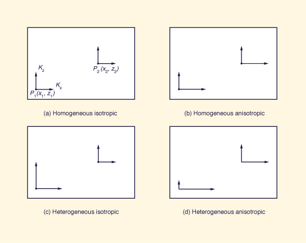
Variability of Hydraulic Conductivity. Soil and rock formations in which hydraulic conductivity is independent of position are said to be homogeneous. Conversely, formations in which hydraulic conductivity is a function of position are said to be heterogeneous.
The formation is said to be isotropic if, at a given point, the hydraulic conductivity is independent of the direction of measurement. On the other hand, if the hydraulic conductivity varies with the direction of measurement, the formation is said to be anisotropic at that point. The four possible combinations of homogeneity, heterogeneity, isotropy, and anisotropy are shown in Fig. 11-4.
Most sedimentary rocks are anisotropic with respect to hydraulic conductivity because the individual particles are not spherical, but they tend to be elongated in a direction parallel to the bedding. This causes the hydraulic conductivity to be greater in a direction parallel to the bedding than in a direction perpendicular to it.
Measured hydraulic conductivities vary by several orders of magnitude. A formation with hydraulic conductivity of 1 m/d would generally be regarded as permeable and likely to be a good aquifer. Conversely, a formation with hydraulic conductivity of less than 10-3 m/d would generally be regarded as impermeable and, therefore, not a good aquifer. However, depending on the intended application, comparisons of hydraulic conductivity (or permeability) are relative. For instance, a formation that is too impermeable for use as an aquifer may at the same time be too permeable for use as a water barrier in the foundation and core of an earth dam.
Figure 11-4 Possible combinations of homogeneity, heterogeneity, isotropy, and anisotropy in porous media [8]. |
Compressibility. Both fluid (water) compressibility and medium (aquifer) compressibility affect groundwater flow.
Assume that an increase in pressure leads to a decrease in volume of a given mass of water. The water compressibility is defined as
|
ΔVw
- _______ Vw β = __________ Δp | (11-10) |
in which β = water compressibility, Vw = volume of a given mass of water, and ΔVw = change in volume caused by a Δp change in pressure. For practical applications, β may be considered to be a constant, since it changes very little over the range of fluid pressures normally encountered in practice. The accepted value of β is 4.4 × 10⁻¹⁰ m2/N (Pa-1).
The compressibility of porous media is quite different from the compressibility of water. Assuming that the compressibility of individual soil grains is negligible, porous media can only be compressed by rearrangement of the soil particles into a tighter packing. The total stress on the media is borne partly by the solid particles forming the granular skeleton and partly by the fluid in pore spaces. The portion of total stress that is borne by solid particles is called the effective stress. Rearrangement of the soil particles is caused by changes in the effective stress and not by changes in total stress. The compressibility of porous media is defined as
|
ΔVT
- _______ VT α = __________ Δσe | (11-11) |
in which α = compressibility of porous media, VT = total volume of the soil mass, and ΔVT = change in volume caused by a Δσe change in effective stress.
The value of α is a function of soil type. Clays have typical α values in the range of 10-6 to 10-8 m2/N; sands, 10-7 to 10-9 m2/N; gravel, 10-8 to 10-10 m2/N; sound rock, 10-9 to 10-11 m2/N [8] . Note that water compressibility is of the same order of magnitude as that of the less compressible geologic materials.
Specific Storage, Transmissivity, and Storativity. Six basic physical properties of fluid (i.e., water) and porous media (soil and rock formation) are needed for the description of saturated groundwater flow; three for the fluid and three for the medium. The water properties are density ρ, absolute viscosity μ, and compressibility β. The porous media properties are porosity n, intrinsic permeability k, and compressibility α. All other parameters describing hydrogeologic properties are based on these; see, for example, the definition of hydraulic conductivity, Eq. 11-9.
Specific storage of a confined aquifer is defined as the volume of water released per unit volume of aquifer per unit decrease in hydraulic head. Compressibility considerations lead to the following expression for specific storage [8]:
| Ss = ρ g (α + n β ) | (11-12) |
in which Ss = specific storage in L -1 units.
The transmissivity of a confined aquifer is defined as follows:
| T = K b | (11-13) |
in which T = transmissivity [L2T -1 units], K = hydraulic conductivity [LT -1units], and b = aquifer thickness [L units]. In SI units, the transmissivity is given in square meters per second. A transmissivity greater than 0.015 m2/s is indicative of a good aquifer, suitable for water well exploitation.
The storativity of a confined aquifer is defined as
| S = Ss b | (11-14) |
in which S = storativity, a dimensionless value. Typical values of storativity vary in the range 0.005 to 0.00005. Given the definition of specific storage, large decreases in hydraulic head over extensive formations are required in order for a confined aquifer to yield substantial amounts of water.
In unconfined aquifers, the concept of specific yield is equivalent to the storativity of confined aquifers. Typical values of specific yield vary in the range 0.01 to 0.30. The higher values of specific yield--as compared to storativity--reflect the fact that releases from an unconfined aquifer represent an actual dewatering of the pore spaces. On the other hand, releases from confined aquifers represent only the secondary effect of aquifer compaction caused by changes in fluid pressure. The favorable yield properties of unconfined aquifers make them more suited to well exploitation.
11.3 EQUATIONS OF GROUNDWATER FLOW
|
|
Depending on whether the flow is steady or unsteady, and saturated or unsaturated, the equations of groundwater flow can be formulated in one of the following three ways:
Steady-state saturated flow,
Transient (i.e., unsteady) saturated flow, and
Transient unsaturated flow.
Equations for steady-state and transient saturated flow are described here. See [8] for details on transient unsaturated flow through porous media.
Steady-State Saturated Flow
The law of conservation of mass for steady-state flow through saturated porous media requires that the net fluid mass flux through a control volume be equal to zero, i.e., the inflow must equal the outflow. This leads to the equation of continuity:
|
∂(ρνx) ∂(ρνy) ∂(ρνz)
________ + ________ + ________ = 0 ∂x ∂y ∂z | (11-15) |
in which the quantities v are specific discharges in three orthogonal directions x, y, and z, respectively. Assuming fluid incompressibility, ρ(x, y, z) is constant, and consequently it can be eliminated from Eq. 11-15. Substitution of Darcy's law in Eq. 11-15 yields:
|
∂(Kx ix) ∂(Ky iy) ∂(Kz iz)
_________ + _________ + _________ = 0 ∂x ∂y ∂z | (11-16) |
in which the quantities K and i are hydraulic conductivities and hydraulic gradients, respectively.
For an isotropic medium, Kx = Ky = Kz = K. For a homogeneous medium, K(x, y, z) is constant, and it can be eliminated from Eq. 11-16. Given ix = ∂h/∂x, iy = ∂h/∂y, and iz = ∂h/∂z, in which h = hydraulic head, Eq. 11-16 reduces to:
|
∂2h ∂2h ∂2h
______ + ______ + ______ = 0 ∂x2 ∂y2 ∂z2 | (11-17) |
Equation 11-17 is the Laplace equation. The solution of this equation is a function h(x, y, z) describing the value of hydraulic head at any point in a three-dimensional flow field. For two-dimensional flow, the third term on the left side of Eq. 11-17 cancels out, and the solution is a function h(x, y).
Transient Saturated Flow
The law of conservation of mass for transient flow through saturated porous media requires that the net fluid mass flux through a control volume be equal to the time rate of change of fluid mass storage within the control volume. Therefore, the equation of continuity, Eq. 11-15, is modified to
|
∂(ρ νx) ∂(ρ νy) ∂(ρ νz) ∂(ρ n)
_________ + _________ + _________ = _________ ∂x ∂y ∂z ∂t | (11-18) |
Assuming that the fluid is incompressible, ρ(x, y, z) is constant, and it can be eliminated from
|
∂(Kx ix) ∂(Ky iy) ∂(Kz iz) ∂n
_________ + _________ + _________ = ______ ∂x ∂y ∂z ∂t | (11-19) |
For an isotropic medium, Kx = Ky = Kz = K. For a homogeneous medium, K(x, y, z) is constant. The time rate of change of porosity can be related to time rate of change of hydraulic head by the following:
|
∂n ∂h
______ = Ss ______ ∂t ∂t | (11-20) |
Therefore, Eq. 11-19 reduces to [14, 15]:
|
∂2h ∂2h ∂2h Ss ∂h
_____ + _____ + _____ = _____ _____ ∂x2 ∂y2 ∂z2 K ∂t | (11-21) |
Equation 11-21 is a diffusion equation, with K/Ss being the hydraulic diffusivity of the aquifer [L2T -1 units]. The solution of this equation is a function h(x, y, z, t) describing the value of hydraulic head in three dimensions at any time. It requires the knowledge of Ss and K or, alternatively, the basic fluid and aquifer properties ρ, μ, α, n, k, and β.
For the special case of a horizontal confined aquifer of thickness b, the third term on the left side of Eq. 11-21 drops out, and with Eqs. 11-13 and 11-14:
|
∂2h ∂2h S ∂h
_____ + _____ = ____ _____ ∂x2 ∂y2 T ∂t | (11-22) |
The solution of this equation is a function h(x, y, t) describing the value of hydraulic head in two dimensions at any time. It requires the knowledge of aquifer storativity S and transmissivity T. The ratio T/S is the hydraulic diffusivity of the aquifer.
11.4 WELL HYDRAULICS
|
|
Well hydraulics describes groundwater flow problems involving discharge to wells. There is a wealth of literature on the subject, including Bear [1], U.S. Bureau of Reclamation [26], and Walton [28]. The classical problem of radial flow to a well is described in this section.
Radial Flow to a Well
Consider an aquifer with the following characteristics:
Horizontal,
Confined between impermeable layers on top and bottom,
Infinite in horizontal extent,
Constant thickness, and
Homogeneous and isotropic.
Furthermore, assume for simplicity: (1) a single pumping well, (2) a constant pumping rate, (3) negligible well diameter relative to the aquifer's horizontal dimensions, (4) well penetration through the entire aquifer depth, and (5) uniform initial hydraulic head throughout the aquifer. In horizontal and vertical coordinates, Eq. 11-22 is the governing equation for this problem, its solution being a function h(x, y, t).
The idealized nature of this problem justifies the assumption of radial symmetry. A sketch of aquifer, pumping well, observational well, and potentiometric surface is shown in Fig. 11-5. The conversion of Eq. 11-22 into radial coordinates, using r = (x2 + y2)1/2, leads to [15]:
|
∂2h 1 ∂h S ∂h
______ + ____ _____ = ____ _____ ∂r 2 r ∂r T ∂t | (11-23) |
in which r is the radial distance from the pumping well to the observational well.
Figure 11-5 Sketch of radial flow to a pumping well. |
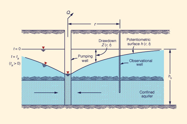
The solution of Eq. 11-23 is a function h(r, t ) describing the potentiometric surface. The uniform initial hydraulic head is h0. For convenience, solutions are often expressed in terms of drawdown, the difference between uniform initial hydraulic head and potentiometric surface:
| Z = h0 - h | (11-24) |
in which Z = drawdown, h0 = uniform initial hydraulic head, and h = hydraulic head (i.e., potentiometric surface elevation).
The assumption of uniform initial hydraulic head throughout the aquifer leads to the following initial condition:
| h (r, 0) = h0 | (11-25) |
for r ≥ 0. Furthermore, assuming no change in hydraulic head at r = ∞, the following boundary condition is obtained:
| h (∞, t ) = h0 | (11-26) |
for t ≥ 0.
Theis Solution
The solution of Eq. 11-23 subject to the given initial and boundary conditions is due to Theis [23]:
|
Q
e-u Z = ______ ∫u∞ ______ du 4πT u | (11-27) |
in which Q = (constant) pumping rate [L 3T -1 units], T = aquifer transmissivity [L 2T -1 units], and u is a dimensionless variable defined as
|
r 2S u = _______ 4T t | (11-28) |
with r = radial distance from pumping well to observational well, S = aquifer storativity (dimensionless), and t = time.
With u defined by Eq. 11-28, the integral in Eq. 11-27 is referred to as the well function W(u), applicable to homogeneous isotropic confined aquifers with full-depth well penetration and at constant pumping rate. Values of W(u) as a function of u are shown in Table 11-1. Equation 11-27 reduces to
|
Q W(u) Z = _________ 4 π T | (11-29) |
| ||||||||||||||||||||||||||||||||||||||||||||||||||||||||||||||||||||||||||||||||||||||||||||||||||||||||||||||||||||||||||||||||||||||||||||||||||||||||||||||||||||||||||||||||||||
Two types of problems can be solved by the Theis method: (1) prediction and (2) identification. In the prediction problem, the pumping rate Q, radial distance r, aquifer transmissivity T, and storativity S are known, and the variation of observational well drawdown Z with time t is sought. In the identification problem, the pumping rate Q, radial distance r, and observational well drawdown versus time data (Z versus t) are known, and the aquifer properties S and T are sought.
The prediction problem can be solved directly with Eqs. 11-28 and 11-29.
For any assumed time t, u is calculated with Eq. 11-28 and used to obtain W(u) from Table 11-1.
Then, Z is calculated with
A variation of the prediction problem is that of the calculation of the cone of depression, or drawdown cone, as shown in Fig. 11-5. In this case, the pumping rate Q and aquifer properties (storativity S and transmissivity T) are known, and the variation of drawdown Z with radial distance r is sought at a fixed time t. For any assumed radial distance r, u is calculated with Eq. 11-28 and used to obtain W(u) from Table 11-1. Then, Z is calculated with Eq. 11-29 for the assumed radial distance r and fixed time t.
The identification problem is solved by a graphical procedure. Eliminating T from Eqs. 11-28 and 11-29 leads to
|
Z Q W(u) _____ = _________ _______ t π r 2 S (1/u) | (11-30) |
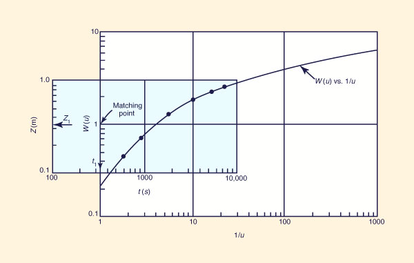
which indicates that the ratio Z /t is proportional to the ratio W(u)/(1/u). The solution is accomplished by the following steps:
-
Using Table 11-1, plot the well function W(u) versus 1/u on logarithmic paper, with 1/u in the abscissas and W(u) in the ordinates.
-
Using the drawdown versus time data for the observational well, plot Z versus t on logarithmic paper, with t in the abscissas and Z in the ordinates.
-
Overlay both plots making sure that they coincide, as shown in Fig. 11-5.
-
Choose a pair of W(u) and 1/u values on the first plot and a pair of matching Z and t values on the second plot. Any pair of W(u) and 1/u is appropriate. For simplicity, the following pair can be chosen: W(u) = 1, and 1/u = 1 (see Fig. 11-6). In this case. the matching pair of Z and t are Z1 and t1. Therefore, using Eqs. 11-29 the transmissivity is:
Q
T = ________
4 π Z1(11-31) Using Eq. 11-28, the storativity is
4T t1
S = _______
r 2(11-32)
For a given radial distance, drawdown increases with increasing time. For a given time, drawdown decreases with increasing radial distance. For a given time and radial distance, drawdown is directly proportional to pumping rate. For a given time, distance, and pumping rate, drawdown is inversely proportional to transmissivity and storativity. Other conditions being constant, low transmissivity results in deep drawdown cones of limited extent, whereas high transmissivity results in shallow cones of wide extent. Likewise, an aquifer of low storativity has a comparatively deeper drawdown cone than an aquifer of high storativity [8].
Figure 11-6 Graphical procedure for Theis solution for radial flow to a well [8]. |
For a detailed discussion of other types of radial flow to a well or wells, including unconfined aquifers, varying pumping rates, multiple-well configurations, and partially penetrating wells, see [8] and [28].
Example 11-1.
Assume a pumping rate Q = 0.00314 m3/s, radial distance from well r = 100 m, aquifer transmissivity T = 0.0025 m2/ s, and aquifer storativity S = 0.001.
Calculate the drawdown after an elapsed time of (a) 1000 s, (b) 10,000 s, and (c) 100,000 s.
For each time t, values of u are calculated with Eq. 11-28.
Corresponding values of W(u) and Z are obtained from Table 11-1 and Eq. 11 -29, respectively.
The results are summarized as follows:
|
Example 11-2.
Assume a pumping rate Q = 0.00314 m3/s, aquifer transmissivity T = 0.0025 m2/s, aquifer storativity S = 0.001, elapsed time t = 10,000 s.
Calculate the drawdown at the following radial distances from the well: (a) 10 m, (b) 100 m, and (c) 200 m.
For each radial distance, values of u are calculated with Eq. 11-28.
Corresponding values of W(u) and Z are obtained from Table 11-1 and Eq. 11-29, respectively.
The results are summarized as follows:
|
11.5 SURFACE-SUBSURFACE FLOW INTERACTION
|
|
The interaction between surface and subsurface flow is central to the study of stream types and baseflow recession. Surface flow occurs in the form of overland flow in the catchments and, subsequently, streamflow in the channel network. Subsurface flow occurs as interflow in the unsaturated zone and as groundwater flow in the saturated zone.
The contribution of subsurface water to surface water is a function of stream type. Depending on whether streams serve as discharge or recharge areas for aquifers, they are classified as (1) effluent, or gaining streams, or (2) influent, or losing streams.
Effluent streams are discharge areas for aquifers. Usually, an aquifer is intersected by the effluent stream, discharging into it. This type of aquifer discharge is distributed along the stream length, in contrast to aquifer discharge that occurs at a point, i.e., a spring. The distributed discharge to effluent streams is referred to as exfiltration, or baseflow, and is typical of humid and subhumid environments where aquifers are at relatively shallow depth.
Influent streams are recharge areas for aquifers, largely due to the high permeability of their channel beds. This type of aquifer recharge-known as channel transmission loss(es) in stream channel routing-is distributed along the stream length and is typical of streams in arid and semiarid regions.
Depending on whether they flow all year, a few days of the year, or seasonally, streams can be further classified as (1) perennial, (2) ephemeral, or (3) intermittent (Section 2.4). Perennial streams are those that flow throughout the year, during both wet and dry weather. Their dry weather flow is largely baseflow, i.e., discharge from groundwater reservoirs. Unlike perennial streams, ephemeral streams are those that flow only in wet weather, i.e., during and immediately following rainfall. In the southwestern United States, ephemeral streams are known as arroyos, washes, or dry washes, and flow approximately 30 d per year on the average. Typically, perennial streams are effluent, whereas ephemeral streams are influent. Furthermore, it is common for ephemeral streams to abstract most or all of their wet-weather flow through channel transmission losses. Intermittent streams are those possessing mixed characteristics, discharging either to or from groundwater reservoirs.
Surface Runoff and Streamflow Generation
Streamflow consists of a combination of surface and subsurface runoff, which can be extremely complex in certain cases. Surface runoff is generated by a gamut of surface and near-surface flow processes, of which some of the most important are:
- Hortonian overland flow
- Saturation overland flow
- Throughflow processes
- Partial-area runoff
- Direct channel interception, and
- Surface phenomena.
Hortonian overland flow [12] describes the process that takes place when rainfall rate exceeds infiltration capacity, usually at the beginning of a storm (or season), when the soil profile is likely to be on the dry side.
Saturation overland flow describes the process that takes place after the soil profile has become saturated, either from antecedent rainfall events or from a sufficient volume of rainfall within the same event. At this point, any additional rainfall, regardless of intensity, will be converted into surface runoff. Saturation overland flow usually occurs during an infrequent storm, or toward the end of a particularly wet season, when the soil is likely to be already wet from prior storms.
Throughflow prevails in heavily vegetated areas with thick soil covers containing less permeable layers, overlying relatively impermeable unweathered bedrock [16]. Throughflow takes place as interflow, or as lateral flow immediately below the ground surface.
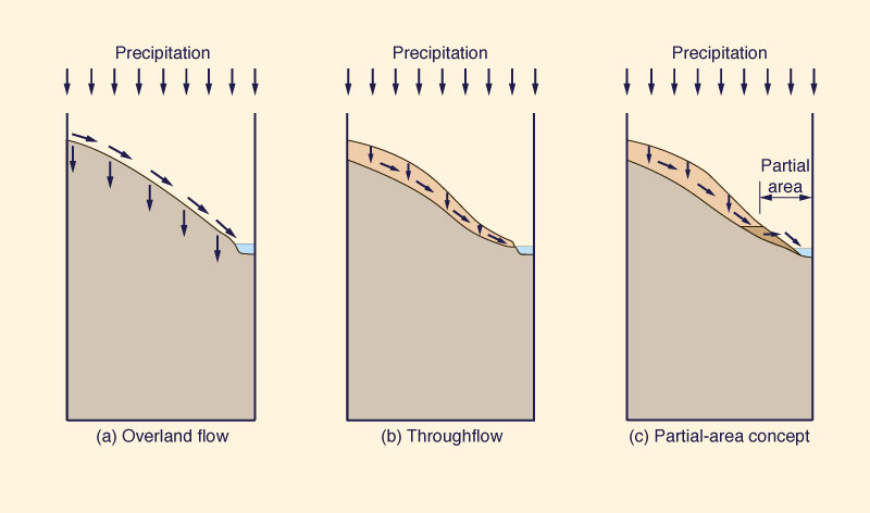
The concept of partial-area runoff developed from the recognition that runoff estimates were improved by assuming that only rainfall on a small and fairly constant part of each drainage basin is able to contribute to direct runoff [16]. Thus, partial-area runoff can be interpreted as a combination of throughflow in the upper hills lopes and saturation overland flow in the lower hillslopes [10, 11, 29].
Direct channel interception refers to the runoff that originates from rainfall falling directly into the channels. This mode of streamflow generation may be important in dense channel networks and certain humid basins.
Surface phenomena includes processes such as crust development, hydrophobic soil layers, and frozen ground, which render the soil surface impermeable, promoting surface runoff and streamflow. For instance, a surface crust may develop following splash erosion in a denuded watershed, adversely affected by human activities or a natural hazard such as fire. Under a specific set of circumstances, including soil type and texture, the silt entrained by splash erosion may deposit on the surface and create a thin crust that eventually reduces the infiltration rate to a negligible level. This mode of surface runoff and streamflow generation is typical of semiarid environments, where surface runoff may take place even though the underlying soil profile, below a relatively thin veneer, remains substantially dry [17, 25].
Hillslope Hydrology and Streamflow Generation
Hillslope hydrology refers to the hydrologic processes taking place on hillslopes. These processes are intrinsically related to streamflow generation. An important question is whether the preferred path of runoff is on the surface, as overland flow, or through the subsurface, by subsurface stormflow, or interflow.
Several theories of hillslope hydrology have been developed, together constituting a spectrum of plausible processes and models [5]. They range from Hortonian theory [12] to throughflow theory [16]. Hortonian theory emphasizes Hortonian overland flow, whereas throughflow theory focuses on interflow processes. Hortonian overland flow is applicable to poorly vegetated slopes with relatively thin soil covers. Throughflow is more apt to explain the processes that take place in heavily vegetated areas with thick permeable soil layers. Between these two extremes lie a variety of models in which runoff is assumed to consists of a mix of Hortonian overland flow, and unsaturated and saturated throughflow.
The partial-area concept is a combination of throughflow in the upper hillslopes and overland flow in the lower hillslopes (Fig. 11-7). Based on field studies, Freeze and Cherry [8] have concluded that most surface runoff hydrographs in humid, vegetated basins originate from not more than 10 percent of the catchment area, and then, are likely to prevail in only 10 to 30 percent of the storms. Betson [2], among others, has documented a substantial improvement in runoff predictions by using the partial-area concept. The size of partial areas is a function of storm depth, rainfall intensity, and antecedent moisture conditions. As a percentage of the total catchment, partial areas in the Southern Appalachians were shown to vary between 5 percent for light-to-moderate storms and 40 percent for heavy storms [2]. With deforestation, the percentage can amount to 80 percent or more. Generally, partial areas may be expected to vary between 5 percent and 20 percent of the total basin [22].
Figure 11-7 Sketch of overland flow, throughflow, and partial-area concepts in hillslope hydrology [5]. |
Refinements of the partial-area concept have led to the variable-source-area model of hillslope hydrology [21, 24]. These variable-source areas are envisioned as comprising low-lying lands adjacent to streams and rivers and concentrated near watershed outlets [3, 7]. Variations in the extent of source areas are dictated by antecedent soil moisture conditions, soil-moisture storage capacity, and rainfall intensity. When the upper soil horizon is saturated, both throughflow and overland flow occur, with eventual exfiltration to stream banks. According to this scheme, the variable-source-area can be interpreted as an expanded stream system, which helps explain the growth in drainage density experienced by small watersheds under heavy rainfall [4].
The variable-source-area model is a dynamic version of the partial-area concept. This dynamism is manifested in soil moisture and runoff changes occurring annually, seasonally, between storms, and during storms. The source areas are largely responsible for overland flow, whereas the remainder of the watershed acts primarily as a reservoir to provide baseflow and to maintain saturation of the source areas [7].
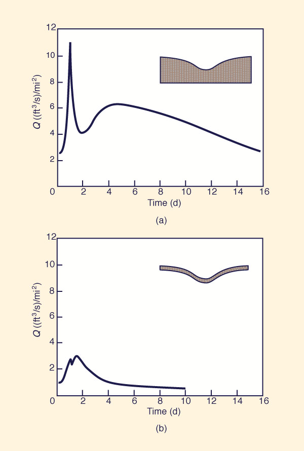
The variable-source-area model visualizes the average storm hydrograph as consisting of (1) rain falling directly onto the channel, and (2) water transmitted rapidly through wet soil adjacent to the stream. The source areas shrink and expand as a function of rainfall amounts and antecedent soil-moisture conditions. In the absence of rainfall, streams are fed to a large extent by moisture moving downslope under unsaturated flow conditions. This downward migration favors the quick release of water from the source areas into the channels during storms. Typical storm hydrographs reflecting the variable-source-area concept are shown in Fig. 11-8.
Figure 11-8 Typical storm hydrographs reflecting variable-source-area concept: |
Hydrograph Separation and Baseflow Recession
The variable-source-area concept has led to increased emphasis on the timing of runoff during and immediately following a storm. This justifies the separation of runoff into two components: (1) quickflow, consisting of fast interflow (subsurface stormflow), overland flow, and rain falling directly on the channels, and (2) baseflow, consisting of slow interflow and groundwater flow.
Hydrograph separation is an established procedure of hydrologic analysis (Section 5.3). It has an important role not only in flood hydrology but also in groundwater hydrology. In flood hydrology, it serves as a means to quantify the relationship between quickflow and baseflow. In groundwater hydrology, it provides information on the nature and behavior of local and regional groundwater regimes.
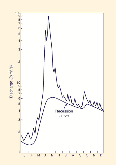
Baseflow Recession. Consider the streamflow hydrograph shown in Fig. 11-9. Flow varies throughout the year, with peaks of approximately 100 m3/s and lows of about 1 m3/s. The smooth line is the baseflow hydrograph or baseflow curve, reflecting the seasonally varying groundwater contributions. The ragged line is the streamflow hydrograph, reflecting the relatively fast response typical of steep catchments with shallow soils of low permeability.
The recession portion of the baseflow curve usually plots as a straight line (or a series of straight lines) on semilogarithmic paper, with discharge plotted on the log scale, as shown in Fig. 11-9. This leads to an equation of the form
| Q = Qo e-t /ts | (11-33) |
in which Q = baseflow at any time t after the starting time
to, Qo = baseflow at to,
and ts = a recession constant known as the time of storage,
defined as the time required for the flow Q to recede to
Figure 11-9 Streamflow hydrograph and baseflow recession curve. |
Other forms of baseflow recession equations are:
| Q = Qo e -αt | (11-34) |
| Q = Qo 10 -t /ts | (11-35) |
| Q = Qo 10 -βt | (11-36) |
| Q = Qo K t | (11-37) |
in which α, β, ts and K are recession constants. The values α and β are positive, and K is generally less than 1. Plotting Eqs. 11-33 to 11-37 on semilogarithmic paper, with discharge on the logarithmic scale, yields a straight line.
From Eqs. 11-33 and 11-37, the relationship between ts and K is
|
1 ts = - _______ ln K | (11-38) |
which leads to
| Q = Qo e (ln K) t | (11-39) |
The integration of Eq. 11-39 between a time corresponding to Qo and a time corresponding to Q leads to:
|
Q - Qo
S = _________ ln K | (11-40) |
in which S = storage volume released from groundwater [L 3 units]. Combining Eqs. 11-38 and 11-40:
| S = ( Qo - Q ) ts | (11-41) |
The volume under the recession curve (from Qo to Q) can be calculated by assuming that as t → ∞,
A historical perspective of baseflow recessions is given by Hall [9].
|
Example 11-3.
Given the following measured recession flows in a certain river:
Calculate:
|
|
Example 11-4.
Given the following measured recession flows in a certain river:
(a) Calculate the time of storage for baseflow, (b) separate the hydrograph into baseflow and quickflow, and (c) calculate the volume released from baseflow in the elapsed 10-h period.
Q9 = Q10 e (1/42) = 81 × 1.024 ≅ 83
in which Δt = 1 h.
To calculate the quickflow values, the baseflow values are subtracted from the total flows.
The calculations are summarized in the following table.
Using Eq. 11-41, the volume released from baseflow is: S =
(101 - 81) ft3/s × 42 h = 840 (ft3/s)-h = 69.4 ac-ft.
|
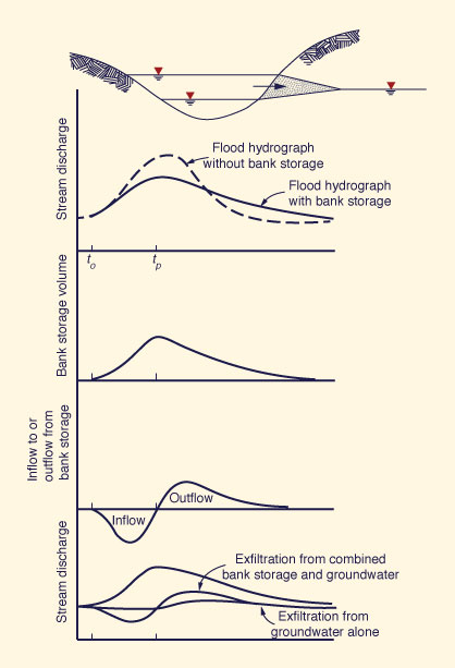
Bank Storage.
A concept closely related to baseflow recession is that of bank storage.
In the upland reaches, subsurface contributions to streamflow generally aid in the buildup of the flood wave.
In the lower reaches, however, bank storage may contribute to flood wave attenuation.
As shown in
Figure 11-10 Effect of bank storage on flood hydrograph magnitude and shape [8]. |
QUESTIONS
|
|
What is the limit between unsaturated and saturated zones in groundwater flow?
What factors determine the feasibility of mining a groundwater reservoir? Explain.
What is an aquifer? An aquiclude? An aquitard?
What are the major differences between confined and unconfined aquifers?
What is a potentiometric surface? A perched aquifer?
Explain the processes of recharge and discharge in unconfined and confined aquifers.
What is specific yield? Specific retention?
What is field capacity? Permanent wilting point?
What is specific discharge? How does hydraulic conductivity differ from intrinsic permeability?
Explain the differences between the compressibility of water and that of porous media.
Define specific storage, transmisivity and storativity. How does the concept of storativity differ from that of specific yield?
What fluid and aquifer properties are needed in the description of saturated groundwater flow?
What additional term is added to the equation of continuity in order to account for transient flow conditions?
What is hydraulic diffusivity in connection with groundwater flow?
What determines whether streams are classified as effluent or influent?
What theories of streamflow generation lie at the two extremes of the spectrum of hillslope hydrologic models?
What is the essential difference between the partial-area and the variable-source-area models of hillslope hydrology?
What runoff components are justified by current theories of hillslope hydrology? Explain.
PROBLEMS
|
|
What is the volume of free-draining water in an unconfined aquifer of surface area A = 130 mi2, thickness b = 300 ft, and specific yield Sy = 0.05?
What is the specific retention of an unconfined aquifer of surface area A = 125 mi2, thickness b = 80 ft, porosity n = 0.30, which can yield 1,536,000 ac-ft of free-draining water?
What is the flow through a porous media with cross-sectional area A = 1250 m2, hydraulic conductivity K = 0.8 × 10⁻⁴ m/s, under a hydraulic gradient i = 0.01?
Derive the exact equivalence between darcys and square centimeters.
What is the hydraulic conductivity of a porous medium with fluid density ρ = 1 g/cm3, intrinsic permeability k = 5 darcys, and fluid absolute viscosity μ = 1 cp.
Show that specific storage Ss has units L-1.
Calculate the storativity of a confined aquifer of thickness b = 50 m, porosity n = 0.05, and compressibility α = 1.0 × 10⁻⁸ Pa-1. Assume fluid density ρ = 1 g/cm3 and compressibility β = 4.4 × 10⁻¹⁰ Pa-1
Calculate the hydraulic diffusivity of an aquifer with the following properties: intrinsic permeability k = 1 darcy, fluid absolute viscosity μ = 1 cp, compressibility α = 1.0 × 10⁻⁸ Pa-1, porosity n = 0.08. Assume fluid compressibility β = 4.4 × 10⁻¹⁰ Pa-1
Calculate the hydraulic diffusivity of an aquifer with storativity S = 0.002, hydraulic conductivity K = 1.0 × 10⁻⁵ cm/s, and thickness b = 100 m.
A well is pumped at the constant rate of Q = 0.004 m3/s in an aquifer of transmissivity T = 0.004 m2/s and storativity S = 0.0005. Calculate the drawdown 24 h after the start of pumping in an observational well located at a distance of 250 m from the pumped well.
A well is pumped at the constant rate of Q = 0.008 m3/s. A match of the well function (W(u) versus 1/u) with drawdown versus time data from an observational well located at a distance of 430 m from the pumped well has produced the following matching values: W(u) = 1, u = 1, Z1 = 0.21 m, and t1 = 1.5 h. Calculate the aquifer transmissivity and storativity.
A well is pumped at a constant rate Q = 0.005 m3/s in an aquifer of transmissivity T = 0.0015 m2/s and storativity S = 0.0005. Calculate the drawdown 24 h after the start of pumping in an observational well located 1000 m from the pumped well.
A well is pumped at a constant rate of 4 L/s. The drawdown in an observational well located at a distance of 150 m from the pumped well has been measured as follows:
Time (min) 0 10 15 30 60 90 120 Drawdown (m) 0 0.16 0.25 0.42 0.62 0.73 0.85 Calculate the transmissivity and storativity of the aquifer.
- Given the following measured recession flows in a certain river:
Time (h) 0 12 24 36 48 Discharge (m3/s) 1000 882 779 687 606 Calculate: (a) the time of storage ts, (b) the volume released from storage in the first 24 h, (c) the volume released from storage in the second 24 h, and (d) the total volume released from storage assuming that the flow eventually recedes back to zero.
- Given the following measured recession flows in a certain stream:
Time (h) 0 1 2 3 4 5 6 Discharge (ft3/s) 1000 920 846 779 716 659 606 Calculate: (a) the time of storage ts, (b) the recession constant K, (c) the volume released from storage between 3 h and 6 h, using both ts (Eq. 11-41) and K (Eq. 11-40), and (d) the total volume released from storage assuming that the flow eventually recedes back to zero, using both Eqs. 11-40 and 11-41.
- Given the following flows measured in the receding limb of a flood hydrograph:
Time (h) 0 1 2 3 4 5 6 7 8 9 10 Flow (m3/s) 32.0 25.2 20.5 17.9 16.1 14.5 13.5 12.9 12.6 12.3 12.0 Calculate: (a) the time of storage for baseflow, (b) the baseflow and quickflow components, (c) the volume released from baseflow in the elapsed 10-h period, and (d) the volume released from baseflow from t = 0 to t = ∞ , assuming that the flow eventually recedes back to zero.
REFERENCES
|
|
Bear, J. (1979). Hydraulics of Groundwater. New York: McGraw-Hill.
Betson, R. P. (1964). "What is Watershed Runoff?" Journal of Geophysical Research, Vol. 69, pp. 1541-155l.
Betson, R. P., and 1. B. Marius. (1969). "Source Areas of Storm Runoff," Water Resources Research, Vol. 5, pp. 574-582.
Carson, M. A., and E. A. Sutton. (1971). "The Hydrologic Response of the Eaton River Basin, Quebec," Canadian Journal of Earth Science, Vol. 8, pp. 102-115.
Chorley, R. J. (1978). "The Hillslope Hydrologic Cycle," in Hillslope Hydrology. M. J. Kirkby, editor. New York: John Wiley, pp. 1-42.
Darcy, H. (1856). "Les Fontaines Publiques de la Ville de Dijon," Paris: Victor Dalmont.
Dunne, T., and R. D. Black. (1970). "Partial Area Contributions to Storm Runoff in a Small New England Watershed," Water Resources Research, Vol. 6, pp. 1296-1311.
Freeze, R. A., and Cherry, J.A. (1979). Groundwater, Englewood Cliffs, N.J.: PrenticeHall.
Hall, F. R. (1968). "Baseflow Recessions-A Review," Water Resources Research, Vol. 4, pp. 973-983.
Hewlett, J. D., and A. R. Hibbert. (1963). "Moisture and Energy Conditions Within a Sloping Soil Mass During Drainage," Journal of Geophysical Research, Vol. 68, pp. 1081-1087.
Hewlett, J. D., and A. R. Hibbert. (1967). "Factors Affecting the Response of Small Watersheds to Precipitation in Humid Areas," Proceedings of the International Symposium on Forest Hydrology, Pennsylvania State University, 1967, pp . 275-290.
Horton, R. E. (1933). "The Role of Infiltration in the Hydrologic Cycle," Transactions, American Geophysical Union, Vol. 14, pp. 446-460.
Hubbert, M. K. (1940). "The Theory of Groundwater Motion," Journal of Geology. Vol. 48, pp. 785-944.
Jacob, C. E, (1940), "On the Flow of Water in an Elastic Artesian Aquifer," Transactions. American Geophysical Union, Vol. 20, pp. 574-586.
Jacob, C. E. (1950). "Flow of Groundwater," in Engineering Hydraulics, Hunter Rouse. editor. New York: John Wiley, pp. 574-586.
Kirkby, M. J., and R. J. Chorley. (1967). "Throughflow, Overland Flow, and Erosion," Bulletin of the International Association of Scientific Hydrology. Vol. 12, pp. 5-21.
Le Bissonais, Y., and Singer, M. J. (1993). "Seal Formation, Runoff, and Interrill Erosion from Seventeen California Soils," Soil Science Society of America Journal, Vol. 57, pp. 224-229.
L'vovich, M. I. (1979). World water resources and their future. Translation of the original Russian edition (1974), American Geophysical Union, Washington, D.C.
Nace, R. L. (1971). "Scientific Framework of World Water Balance," UNESCO Technical Papers in Hydrology, No.7.
Price, M. (l985). Introducing Groundwater. London: Allen and Unwin.
Ragan, R. M. (1968). "An Experimental Investigation of Partial Area Contributions," Proceedings of the General Assembly, Internatzonal Association for ScientifIc Hydrology, Berne, Publication 76, pp. 241-249.
Tennessee Valley Authority. (1966). "Cooperative Research Project in Western North Carolina, Annual Report, Water Year 1964-65," Knoxville, Tennessee.
Theis, C. V. (1935). "The Relation between the Lowering of the Piezometric Surf!lce and the Rate of Duration of Discharge of a Well Using Groundwater Storage," Transactions, American Geophysical Union, pp. 519-524 .
Tsukamoto, Y. (1963). "Storm Discharge from an Experimental Watershed," Journal of the Japanese Society of Forestry. Vol. 45, No.6, pp. 186-190.
U.S. Department of Agriculture. (1940). "Influences of Vegetation and Watershed Treatments of Runoff, Silting, and Erosion, A Progress Report of Research" Misc. Pub. No. 397, July.
U.S. Dept. of Interior, Bureau of Reclamation. (1977). Groundwater Manual.
U.S. Water Resources Council, Hydrology Committee. (1980). "Essentials of Groundwater Hydrology Pertinent to Water Resources Planning," Bulletin 16, (revised).
Walton, W. C. (1970). Groundwater Resource Evaluation. New York: McGraw-Hill.
Wenzel, L. K. (1942). "Methods for Determining Permeability of Water-Bearing Materials," U.S. Geological Survey Water Supply Paper 887.
Whipkey, R. Z. (1965). "Subsurface Stormflow from Forested Slopes," Bulletin of the International Association for Scientific Hydrology, Vol. 10, No.2, pp. 74-85.
World Water Balance and Water Resources of the Earth (1978). Committee for the International Hydrological Decade, UNESCO, Paris, France.
Chorley, R. J. (1978). "The Hillslope Hydrologic Cycle," in Hillslope Hydrology. M.J. Kirkby, editor. New York: John Wiley, pp. 1-42.
Freeze, R. A., and Cherry, J. A. (1979). Groundwater. Englewood Cliffs, N.J.: Prentice- Hall.
Horton, R. E. (1933). "The Role of Infiltration in the Hydrologic Cycle," Transactions, American Geophysical Union, Vol. 14, pp. 446-460.
Hubbert, M. K. (1940). "The Theory of Groundwater Motion," Journal of Geology, Vol. 48, pp. 785-944.
| http://engineeringhydrology.sdsu.edu |
|
201017 |