|
|
|
CHAPTER 8: RESERVOIR ROUTING |
|
"The kinematic wave routing schemes use a unique stage-discharge relation, so that their differential equation should provide pure translation of the flood wave, without attenuation. However,
it is observed that, in practical calculations using these methods, an attenuation is in fact obtained." Michael B. Abbott (1976) |
|
This chapter is divided into five sections. Section 8.1 discusses general concepts of storage routing, the foundation of the remaining sections. Section 8.2 discusses linear reservoirs and their use in simulated reservoir routing. Section 8.3 describes the storage-indication method and its use in actual reservoir routing with uncontrolled outflow. Section 8.4 discusses reservoir routing with controlled outflow. Section 8.5 discusses detention basins and detention basin design. |
8.1 STORAGE ROUTING
|
|
Reservoirs
In many applications of engineering hydrology, it is necessary to calculate the variation of flows in time and space. These applications include reservoir design, design of flood control structures, flood forecasting, and water resources planning and analysis.
A reservoir is a natural or artificial feature which stores incoming water and releases it at regulated rates. Surface-water reservoirs should be distinguished from groundwater reservoirs; the latter store groundwater. Surface-water reservoirs store water for diverse uses, including hydropower generation, municipal and industrial water supply, flood control, irrigation, navigation, fish and wildlife management, water quality, and recreation. This chapter deals with reservoir routing in surface-water reservoirs.
Reservoir routing uses mathematical relations to calculate outflow from a reservoir once the inflow, initial conditions, reservoir characteristics, and operational rules are known. The classical approach to reservoir routing is similar to that of the storage concept described in Chapter 4. Reservoir routing techniques based on the storage concept are referred to as hydrologic routing methods, or storage routing methods, to distinguish them from the more complex hydraulic routing method. The latter uses principles of mass and momentum conservation to obtain detailed solutions for discharges and stages throughout the reservoir [2]. In practice, however, nearly all applications of reservoir routing have used the storage concept.
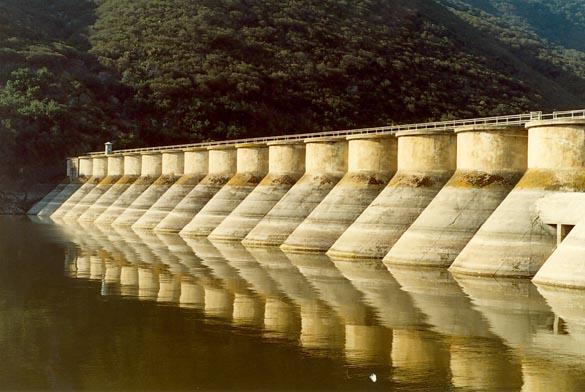
Reservoirs can be of widely differing sizes. They can range from small detention ponds designed to diffuse flood flows from developed urban sites, to very large reservoirs encompassing substantial segments of large rivers (Fig. 8-1). For a single reservoir, inflow is dependent on the upstream flows, whether the latter have been modified by human action or not. Outflow, however, may be of the following types: (1) uncontrolled, (2) controlled, or (3) a combination of both. Uncontrolled outflow is not subject to operator intervention; for example, the case of an ungated overflow spillway. On the other hand, controlled outflow is subject to operator intervention, as in the case of a gated outlet pipe or spillway. In certain instances, reservoirs are outfitted with a combination of controlled and uncontrolled outflow devices or structures.
Figure 8-1 Lake Hodges Dam, in San Diego, California, in operation since 1918. |
Detention ponds and small flood-retention reservoirs are typical examples of uncontrolled outflow. In these cases, an ungated overflow spillway (or, alternatively, a gated spillway that is kept fully open during the flood season) serves as the outflow structure. From a hydraulic standpoint (Chapter 4), outflow from this type of reservoir is solely a function of reservoir stage (pool level, or water surface elevation).
There are two types of reservoir routing with uncontrolled outflow: (1) simulated, and (2) actual. Simulated reservoir routing uses mathematical relations to mimic natural diffusion processes in the computational model (or hydrologic software). A typical example of simulated reservoir routing is the linear reservoir method, which is extensively used in catchment routing (Chapter 10).
Actual reservoir routing refers to the routing through a planned or existing reservoir, either for design or operational purposes. In this case, the outflow characteristics are determined by the geometric properties of the reservoir and the hydraulic properties of the outflow structure(s). The most widely used method of actual reservoir routing with uncontrolled outflow is the storage-indication method.
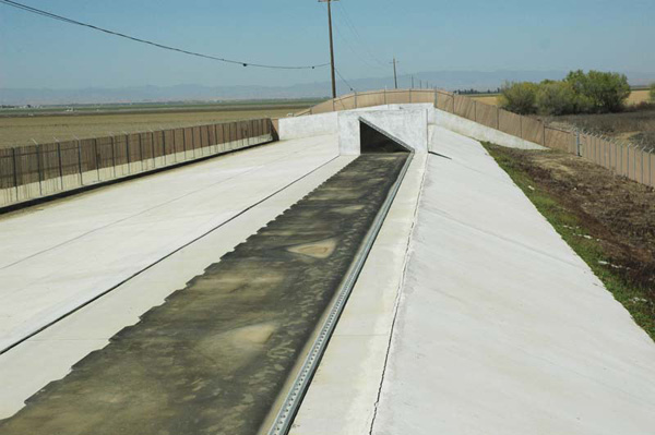
In a reservoir with controlled outflow, gates are used for the purpose of regulating flow through the outlet structure(s) (Fig. 8-2). The gates are operated following established operational rules. These rules determine the relation between inflow, outflow, and reservoir storage volume, taking into account the daily, monthly, or seasonal downstream water demands. The latter may include a minimum instream flow requirement for water quality or fisheries management. Many large reservoirs operate with controlled outflow conditions.
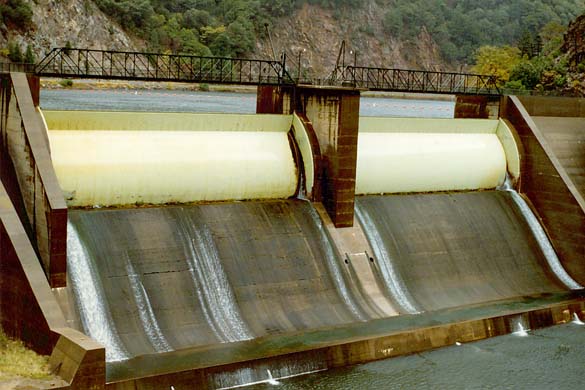
Figure 8-2 Rubber-gated spillway, Arroyo Pasajero sediment retention basin, near Coalinga, California. |
In certain cases, outflow may be a combination of controlled and uncontrolled types--for instance, when the reservoir features a combined regulated outflow and emergency spillway designed to operate only above a certain pool level. Flow through an emergency overflow spillway is usually of the uncontrolled type, the outflow being determined solely by the hydraulic properties of the spillway, without the need for operator intervention.
Storage Routing
The storage concept is well established in flow-routing theory and practice. Storage routing is used not only in reservoir routing but also in stream channel and catchment routing (Chapters 9 and 10). Techniques for storage routing are invariably based on the differential equation of water storage. This equation is founded on the principle of mass conservation, which states that the change in flow per unit length in a control volume is balanced by the change in flow area per unit time. In partial differential form:
|
∂Q ∂A ____ + ____ = 0 ∂x ∂t | (8-1) |
in which Q = flow rate, A = flow area, x = space (length), and t = time.
The differential equation of storage is obtained by lumping spatial variations. For this purpose, Eq. 8-1 is expressed in finite increments:
|
ΔQ ΔA _____ + _____ = 0 Δx Δt | (8-2) |
With ΔQ = O - I, in which O = outflow and I = inflow; and ΔS = ΔA Δx , in which ΔS = change in storage volume, Eq. 8-2 reduces to:
|
ΔS I - O = _____ Δt | (8-3) |
in which inflow, outflow, and rate of change of storage are expressed in L3T-1 units. Furthermore, Eq. 8-3 can be expressed in differential form, leading to the differential equation of storage:
|
dS I - O = _____ dt | (8-4) |
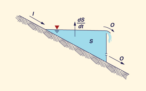
Equation 8-4 implies that any difference between inflow and outflow is balanced by a change of storage in time (Fig. 8-3). In a typical reservoir routing application, the inflow hydrograph (upstream boundary condition), initial outflow and storage (initial conditions), and reservoir physical and operational characteristics are known. Thus, the objective is to calculate the outflow hydrograph for the given initial condition, upstream boundary condition, reservoir characteristics, and operational rules.
Figure 8-3 Inflow, outflow, and change of storage in a reservoir. |
Storage-Outflow Relations
Unlike in an ideal channel for which storage is a function of both inflow and outflow, in an ideal reservoir storage is a function only of outflow (Section 4.2). The relationship between storage and outflow can be expressed in the following general form:
| S = f (O ) | (8-5) |
A common relationship between outflow and storage is the following power function:
| S = K O n | (8-6) |
in which K = storage coefficient and n = exponent. For n = 1, Eq. 8-6 reduces to the linear form:
| S = K O | (8-7) |
in which K is a proportionality constant or linear storage coefficient, which has the units of time (T ).
Real reservoirs usually have a nonlinear storage-outflow relationship; therefore, Eq. 8-6 is applicable to planned or existing reservoirs. Exceptions are the cases where the storage-outflow relation is indeed linear, as in the case of the proportional weir. The latter is used in connection with irrigation diversions or measurement of small sanitary flows.
Simulated reservoirs are usually of the linear type (Eq. 8-7), although nonlinear reservoirs have also been used in simulation. The use of several linear reservoirs in series leads to a cascade of linear reservoirs, a mathematical procedure that is useful in routing, particularly in catchment routing (Chapter 10). For linear reservoirs, the constant K is the linear storage coefficient. Increasing the value of K increases the amount of storage simulated by the system. In other words, greater values of K result in increased outflow hydrograph diffusion.
For routing in actual reservoirs, the nonlinear properties of the storage-outflow relation must be determined in advance. Outflow from an actual reservoir will depend on whether the flow is discharged through either closed conduit(s), overflow spillway(s), or a combination of the two. A general hydraulic outflow formula is the following:
| O = Cd Z H y | (8-8) |
in which
O = outflow;
Cd = discharge coefficient;
Z = variable representing either (1) cross-sectional area A for a free-outlet closed conduit, or (2) crest length L for a free-surface overflow spillway;
H = hydraulic head, taken either (1) above outlet elevation for a closed conduit, or (2) above spillway crest for an overflow spillway; and
y = exponent of the rating.
Theoretical values of discharge coefficient Cd and rating exponent y are determined using hydraulic principles. For the free-outlet closed conduit, the conservation of energy between reservoir pool and outlet elevations (neglecting entrance and friction losses) leads to:
|
V 2 H = ____ 2g | (8-9) |
in which V = mean velocity, and g = gravitational acceleration. Therefore, the outflow is:
| O = ( 2gH )1/2 A | (8-10) |
Comparing Eq. 8-10 with Eq. 8-8, it follows that y = 1/2, with Cd = 4.43 in SI units and Cd = 8.02 in U.S. customary units. In practice, these theoretical values of discharge coefficient are reduced by about 30 percent to account for flow contraction and entrance and friction losses.
For an ungated overflow spillway, the critical flow condition in the vicinity of the crest leads to:
| O = [ g (2/3) H ]1/2 [ (2/3)H ] Z | (8-11) |
which reduces to:
| O = (2/3)[ (2/3)g ]1/2 Z H 3/2 = 0.5443 (g)1/2 L H 3/2 | (8-12) |
Comparing Eq. 8-12 with Eq. 8-8, it follows that y = 3/2. Furthermore, the discharge coefficient in SI units, with g = 9.81 m/s2, is: Cd = 1.70. In U.S. customary units, with g = 32.17 ft/s2: Cd = 3.09.
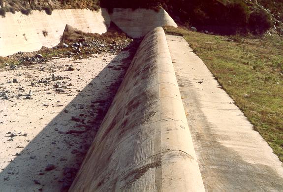
In practice, the discharge coefficient of an overflow spillway varies with hydraulic head, depending on the shape of the spillway crest; see, for example, Fig. 8-4.
Figure 8-4 Ogee spillway of El Capitan Dam, in San Diego, California, completed in 1934. |
In the proportional or Sutro® weir, the cross-sectional flow area, above the rectangular section, grows in proportion to the half-power of the hydraulic head
Figure 8-5 Proportional weir. |
8.2 LINEAR RESERVOIRS
|
|
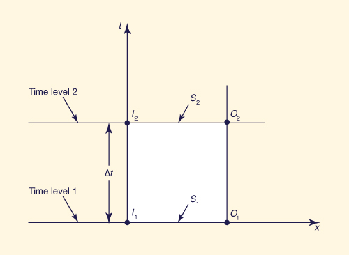
Equation 8-4 can be solved by analytical or numerical means. The numerical approach is usually preferred because it can account for an arbitrary inflow hydrograph. The solution is accomplished by discretizing Eq. 8-4 on the xt plane, a graph showing the values of a certain variable in discrete points in time and space (Fig. 8-6).
Figure 8-6 shows two consecutive time levels, 1 and 2, separated between them an interval Δt, and two spatial locations depicting inflow and outflow, with the reservoir located between them. The discretization of Eq. 8-4 on the xt plane leads to:
|
I1 + I2 O1 + O2 S2 - S1 _________ - __________ = _________ 2 2 Δt | (8-13) |
in which I1 = inflow at time level 1; I2 = iriflow at time level 2; O1 = outflow at time level 1; I2 = outflow at time level 2; S1 = storage at time level 1; S2 = storage at time level 2; and Δt = time interval. Equation 8-13 states that between two time levels 1 and 2 separated by a time interval Δt, average inflow minus average outflow is equal to change in storage.
Figure 8-6 Discretization of storage equation in xt plane. |
For linear reservoirs, Eq. 8-7 is the relation between storage and outflow. Therefore:
| S1 = K O1 | (8-14a) |
and
| S2 = K O2 | (8-14b) |
in which K is the storage constant.
Substituting Eqs. 8-14 into 8-13, and solving for O2:
| O2 = C0 I2 + C1 I1 + C2 O1 | (8-15) |
in which C0, C1 and C2 are routing coefficients defined as follows:
|
Δt /K C0 = ________________ 2 + ( Δt /K ) | (8-16) |
| C1 = C0 | (8-17) |
|
2 - ( Δt /K ) C2 = _________________ 2 + ( Δt /K ) | (8-18) |
Since C0 + C1 + C2 = 1, the routing coefficients are interpreted as weighting coefficients. These routing coefficients are a function of Δt /K, the ratio of time interval to storage constant. Values of the routing coefficients as a function of Δt /K are given in Table 8-1. The linear reservoir routing procedure is illustrated by Example 8-1.
| ||||||||||||||||||||||||||||||||||||||||||||||||||||||||||||||||||||||||||||||||||||||||||||||||||||||||||||||||||||||||||||||||||||||||||||||||||||||||||||||||||||||||||||||||||||||||||||||||||||||||||||||||||||||||||||||||||||||||||||||||||||||||||||||
Figure 8-7 Linear reservoir routing: Example 8-1. |
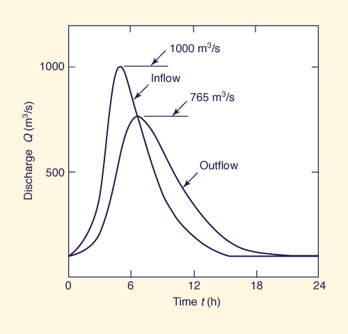
The reservoir exerts a diffusive action on the flow, with the net result that peak flow is attenuated and time base is increased. In the linear reservoir case, the amount of attenuation is a function of Δt /K. The smaller this ratio, the greater the amount of attenuation exerted by the reservoir. Conversely, large values of Δt /K cause less attenuation. Values of Δt /K greater than 2 can lead to negative attenuation (see Table 8-1). This amounts to amplification; therefore, values of Δt /K greater than 2 are not used in reservoir routing.
|
A distinct characteristic of reservoir routing is the occurrence of peak outflow at the time when inflow equals outflow; see Fig. 8-7. Since outflow is proportional to storage according to Eq. 8-7, peak outflow must correspond to maximum storage. Since storage ceases to increase when outflow equals inflow, maximum storage and peak outflow must occur at the time when inflow and outflow coincide.
Another characteristic of reservoir routing is the immediate outflow response, with no apparent lag between the start of inflow and the start of outflow;
see, for instance, |
In effect, the celerity of short surface waves is [4]:
| c = u ± (g h)1/2 | (8-19) |
in which u = mean velocity, and h = flow depth.
Dividing Eq. 8-19 by u, and considering only the positive dimensionless celerity c' :
|
c c' = ___ = 1 + (1/F) u | (8-20) |
in which the Froude number F = u /(g h)1/2.
In the case of a reservoir, the water surface slope Sw ≅ 0,
the mean velocity
8.3 STORAGE INDICATION
|
|
The storage indication method is also known as the modified Puls method [1]. It is used to route streamflows through actual reservoirs, for which the relationship between outflow and storage is usually of a nonlinear nature.
The method is based on the differential equation of storage, Eq. 8-4. The discretization of this equation on the xt plane (Fig. 8-6) leads to Eq. 8-13. In the storage indication method, Eq. 8-13 is transformed to its equivalent form:
|
2 S2
2 S1 ______ + O2 = I1 + I2 + ______ - O1 Δt Δt | (8-21) |
in which the unknown values (S2 and O2) are on the left side of the equation and the known values (inflows, initial outflow and storage) are on the right side. The left side of Eq. 8-21 is known as the storage indication quantity.
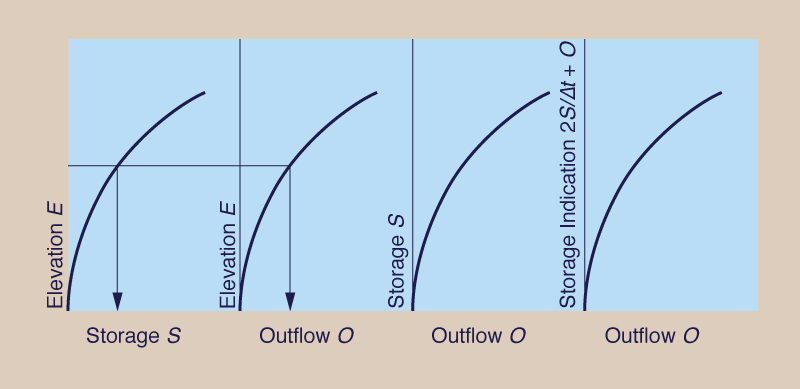
In the storage indication method, it is first necessary to assemble geometric and hydraulic reservoir data in suitable form. For this purpose, the following curves are prepared (Fig. 8-8):
- Elevation-storage,
- Elevation-outflow,
- Storage-outflow, and
- Storage indication-outflow.
For computer applications, these curves are replaced by digitized tables.
Figure 8-8 Geometric and hydraulic data for the storage indication method. |
The elevation-storage relation is determined based on topographic information. The minimum elevation is that for which storage is zero, and the maximum elevation is the minimum elevation of the dam crest.
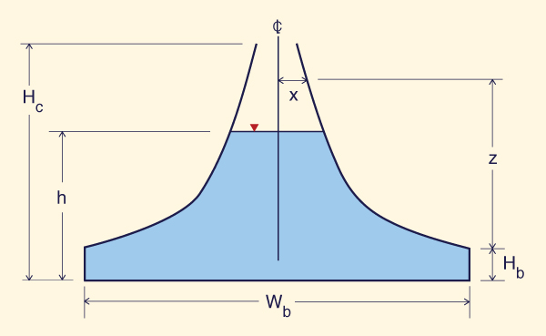
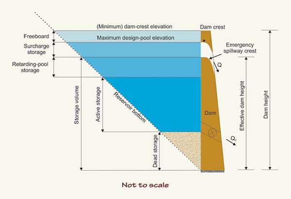
The elevation-outflow relation is determined based on the hydraulic properties of the outlet works, either closed conduit, overflow spillway, or a combination of the two. In the typical application, the reservoir pool elevation provides a head over the outlet or spillway crest, and the outflow can be calculated using an equation such as Eq. 8-8. When routing floods through emergency spillways, storage is alternatively expressed in terms of surcharge storage, i.e., the storage above a certain level, usually the emergency spillway crest elevation (Fig. 8-9).
Figure 8-9 Definition sketch for reservoir storage volumes. |
Elevation-storage and elevation-outflow relations lead to the storage-outflow relation. In turn, the storage-outflow relation is used to develop the storage indication-outflow relation (Fig. 8-8). The storage indication variable is the left-hand side of Eq. 8-21. In general, the storage indication quantity is [(2S/Δt) + O], with S = storage, O = outflow, and Δt = time interval. To develop the storage indication-outflow relation, it is first necessary to select a time interval such that the resulting linearization of the inflow hydrograph remains a close approximation of the actual nonlinear shape of the hydrograph. For smoothly rising hydrographs, a minimum value of tp/Δt = 5 is recommended, in which tp is the time-to-peak of the inflow hydrograph. In practice, a computer-aided calculation would normally use a much greater ratio.
Once the data has been prepared, Eq. 8-21 is used to perform the reservoir routing.
|
The storage-indication procedure consists of the following steps:
|
The computational procedure is illustrated in Example 8-2 using the same data as in Example 8-1. The results of Example 8-2 confirm that the storage indication method is applicable to linear reservoir data.
Example 8-3 illustrates the application of the storage indication method to an actual reservoir featuring a nonlinear storage-outflow relation.
Example 8-2.
Use the data in Example 8-1 to perform a reservoir routing by the storage indication method.
Since K = 2 h and the reservoir is linear, the outflow-storage relation is the following:
in which outflow O is in cubic meters per second and storage S is in (cubic meters per second)-hour for computational convenience.
Selecting Δt = 1 h as in the previous example, the storage indication variable is [(2S/Δt + O] = 5 (O), from which
The calculations are shown in Table 8-3.
At t = 0, the counter is set at n = 1, the outflow (Col. 5) is 100 m3/s (baseflow), and the storage indication quantity (Col. 4) is: 100 × 5 = 500 m3/s.
Therefore, Col. 3 is: 500 - (2 × 100) = 300 m3/s.
For n = 1, between t = 0 and t = 1, Eq. 8-21 is used to calculate the storage indication at
The counter is incremented by 1 and the recursive procedure is continued until the outflow hydrograph ordinate (Col. 5) is within 5% of baseflow discharge (100 m3/s).
The results of Table 8-3, Col. 5 are confirmed to be the same as those of Table 8-2, Col. 6.
ONLINE CALCULATION.
Using ONLINE ROUTING02, the answer
is essentially the same as that of Col. 5, Table 8-3.
| ||||||||||||||||||||||||||||||||||||||||||||||||||||||||||||||||||||||||||||||||||||||||||||||||||||||||||||||||||||||||||||||||||||||
Example 8-3.
The design of an emergency spillway calls for a broad-crested weir of width L = 10 m; rating coefficient Cd = 1.7;
and rating exponent 1.5 (Eq. 8-12).
The spillway crest is at elevation 1070 m.
Above this level, the reservoir walls can be considered to be vertical, with a surface area of 100 ha.
The dam crest is at elevation 1076 m.
Baseflow is 17 m3/s, and initially the reservoir level is at elevation 1071 m.
Route the following design hydrograph through the reservoir.
What is the maximum pool elevation reached?
The calculations of the storage indication function are shown in Table 8-4.
Column 1 shows water surface elevations, from 1070 to 1076.
Column 2 shows the head above spillway crest.
Column 3 shows the outflows, calculated by the following formula:
Column 4 shows the storage volumes in cubic meters above spillway crest elevation (i.e.,
surcharge storage), calculated as the product of reservoir surface area (100 ha) times head above spillway crest.
Column 5 shows storage volumes in (cubic meters per second)-hour.
A time interval Δt = 1 h is appropriate for this example.
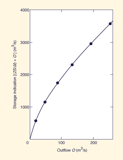
Column 6 shows the storage indication quantities [(2S/ Δt + O ], in m3/s.
Figure 8-10 shows the storage indication versus outflow relation (storage-indication function).
The routing is summarized in Table 8-5.
Column 1 shows time.
Column 2 shows the inflow hydrograph.
Column 3 shows the quantity [ (2S / Δt ) - O ].
Column 4 shows the storage indication
quantity [ (2S / Δt ) + O ].
Column 5 shows the calculated outflow.
The recursive procedure is the same as in the previous example.
The initial outflow (baseflow) is 17 m3/s; the initial storage indication value is 572.56 m3/s; the initial value of Col. 3 is 538.56 m3/s.
The next storage indication value is 17 + 20 + 538.56 = 575.56 m3/s, which through Fig. 8-5 leads to an outflow of 17.1 m3/s.
The recursive procedure continues until the outflow has substantially reached baseflow conditions.
To calculate the maximum pool elevation, use Eq. 8-24 and solve for H with the peak outflow value of 72.9 m3/s.
This results in a maximum head of 2.64 m above the spillway crest.
Therefore, the maximum pool elevation is: 1070.0 + 2.64 = 1072.64 m.
ONLINE CALCULATION.
Using ONLINE ROUTING03, the answer
is very close to that of Col. 5, Table 8-5.
| ||||||||||||||||||||||||||||||||||||||||||||||||||||||||||||||||||||||||||||||||||||||||||||||||||||||||||||||||||||||||||||||||||||||||||||||||||||||||||||||||||||||||||||||||||||||||||||||||||||||||||||||||||||||||||||||||||||||||||||||||||||||||
Figure 8-10 Storage indication function: Example 8-3. |
8.4 CONTROLLED OUTFLOW
|
|
Most large reservoirs have some type of outflow control, wherein the amount of outflow is regulated by gated spillways. In this case, the prescribed outflow is determined by both hydraulic conditions and operational rules. Operational rules take into account the various uses of water. For instance, a multipurpose reservoir may be designed for hydropower generation, flood control, irrigation, and navigation.
For hydropower generation, the reservoir pool level is kept within a narrow range, usually close to the optimum operating level of the installation. On the other hand, flood-control operation may require that a certain storage volume be kept empty during the flood season in order to receive and attenuate the incomIng floods. Flood-control operations also require that the reservoir releases be kept below a certain maximum, usually taken as the flow corresponding to bank-full stage. Irrigation requirements may vary from month to month depending on the consumptive needs and crop patterns. For navigation purposes, outflow should be a nearly constant value that will ensure a minimum draft downstream of the reservoir.
Reservoir operational rules are designed to take into account the various water demands. These are often conflicting and, therefore, compromises must be reached. Multipurpose reservoirs allocate reservoir volumes to the different uses. In this way, operational rules may be developed to take into account the requirements of each use (Fig. 8-11). In general, outflow from a reservoir with gated outlets is determined by prescribed operational policies. In tum, the latter are based on the current level of storage, incoming flow, and downstream flow requirements.
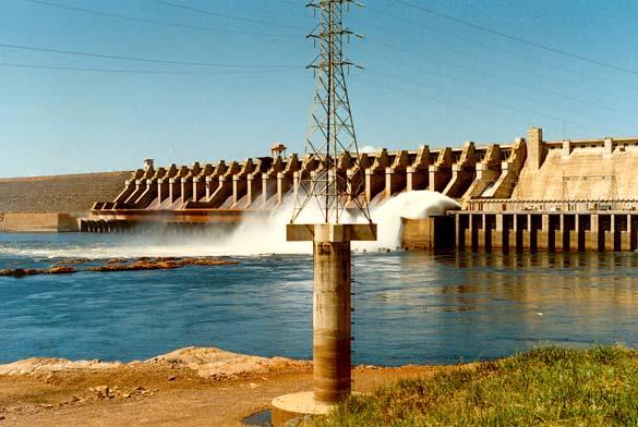
Figure 8-11 Tucurui Dam, on the Tocantins River, Para, Brazil. |
The differential equation of storage can be used to route flows through reservoirs with controlled outflow (Fig. 8-12). In general, the outflow can be either: (1) uncontrolled (ungated), (2) controlled (gated), or (3) a combination of controlled and uncontrolled. The discretized equation, including controlled outflow, is:
|
I1 + I2 O1 + O2 S2 - S1 _________ - __________ - Ōr = _________ 2 2 Δt | (8-25) |
in which Ōr is the mean regulated outflow during the time interval Δt. Equation 8-23 can be expressed in storage indication form:
|
2 S2
2 S1 ______ + O2 = I1 + I2 + ______ - O1 - 2 Ōr Δt Δt | (8-26) |
With Ōr known, the solution proceeds in the same way as with the uncontrolled outflow case. In the case where all the outflow is controlled, Eq. 8-23 reduces to:
|
2 S2
2 S1 ______ = I1 + I2 + ______ - 2 Ōr Δt Δt | (8-27) |
Furthermore, Eq. 8-27 is expressed as follows:
|
Δt S2 = S1 + ______ (I1 + I2) + - (Δt) Ōr 2 | (8-28) |
by which the storage volume can be updated based on average inflows and mean regulated outflow. Other requirements, such as estimates of reservoir evaporation where warranted (i.e., in semiarid and arid regions) may be implemented to properly account for the storage volumes.
Figure 8-12 Cresta Dam, on the North Fork Feather River, Plumas County, California. |
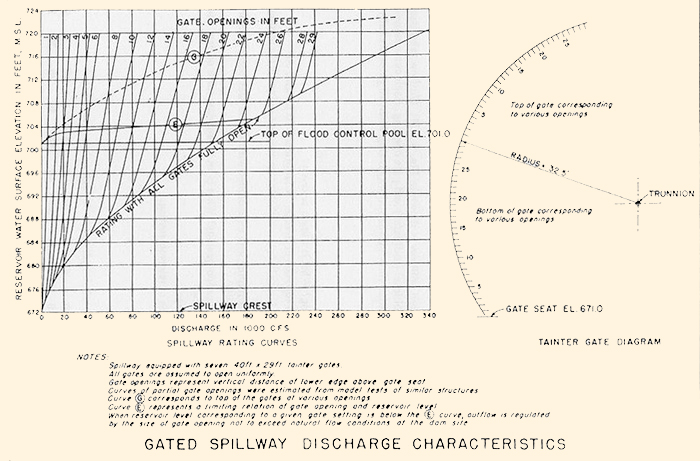
Rating of Gated Spillways
A typical rating of a gated spillway is shown in Fig. 8-13 [5]. Outflow discharge (abscissas) is a function of reservoir water surface elevation (ordinates) and gate opening. Each curve represents a different gate opening. Also shown is the spillway rating when all gates are fully open.
Figure 8-13 Example of rating of gated spillway [Click here ⇔ ⇔ to enlarge the figure] [5].. |
8.5 DETENTION BASINS
|
|
As rural areas become urbanized, storm runoff increases in both peak and volume. The paving of formerly rural lands effectively decreases hydrologic abstractions, resulting in marked increases in storm runoff volume. To compound the problem, paving decreases friction and accelerates runoff concentration, shortening the time of concentration and increasing peak flows (Section 2.4). An accumulation of many of these changes in short-term hydrologic response at the local level may affect the magnitude and frequency of floods at downstream sites.
Local governments are enacting regulations to control and manage changes in short-term hydrologic response which may be attributed to land development. These changes are often referred to as hydromodification. A typical control strategy requires that post-development peak flows do not exceed pre-development peak flows, for one or more storm frequencies at specified sites. This is accomplished by storing the storm water to decrease the calculated post-development peak flow (prior to attenuation) to a level dictated by local regulation, usually the pre-development peak flow.
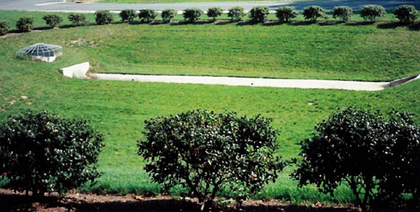
A detention basin (Fig. 8-14) is a small reservoir, built typically in an urban setting, designed to hold and diffuse storm runoff to mitigate and reduce regional downstream floods and channel erosion. As societies learn to recognize the role of anthropogenic activities on floods, attention is increasingly being paid to flood detention and retention as an effective flood control strategy.
Figure 8-14 A detention basin in an urban area. |
The detention basin is a widely used method for controlling peak discharge in urban areas. It is generally the least expensive and most reliable of the measures that are usually considered for controlling storm runoff [6]. It can be designed to fit a wide variety of sites and can accomodate multiple-outlet spillways to meet specific requirements for multifrequency control of outflow. The design of a detention basin, like that of any reservoir, calls for routing of the inflow hydrograph through the structure to determine the required storage volume and the dimensions of the outlet structures. Proprietary (commercial) and nonproprietary (government) software packages are available for routing floods through detention basins, either as stand-alone structures, or as part of a network of detention basins, channels, and other structural flood control measures.
TR-55 Storage Volume for Detention Basins
The USDA Natural Resources Conservation Service (NRCS) has developed a method to estimate storage volume for detention basins. The method, referred to as TR-55 detention basin, is recommended for preliminary design, in lieu of more elaborate routing techniques. The method provides an expedient way to estimate the effects of temporary detention on peak discharges. It may be adequate for final design of small detention basins.
The following are defined:
- Storm runoff volume Vr
- Peak inflow discharge Qi
- Peak outflow discharge Qo
- Detention basin storage volume Vs .
The storm runoff volume Vr is obtained by multiplying the storm runoff depth times the catchment area. The peak inflow discharge Qi is taken as the post-development peak flow, prior to attenuation with the detention basin. The peak inflow discharge is calculated with the TR-55 graphical or tabular methods (Chapter 5) [6]. The peak outflow discharge Qo is normally taken as the pre-development peak flow.
Figure 8-15 is used to estimate Vs when Vr, Qi and Qo are known. Alternatively, this figure can be used to estimate Qo when Vs, Vr, and Qi are known.
Figure 8-15 TR-55 design chart to calculate storage volume for a detention basin [6]. |
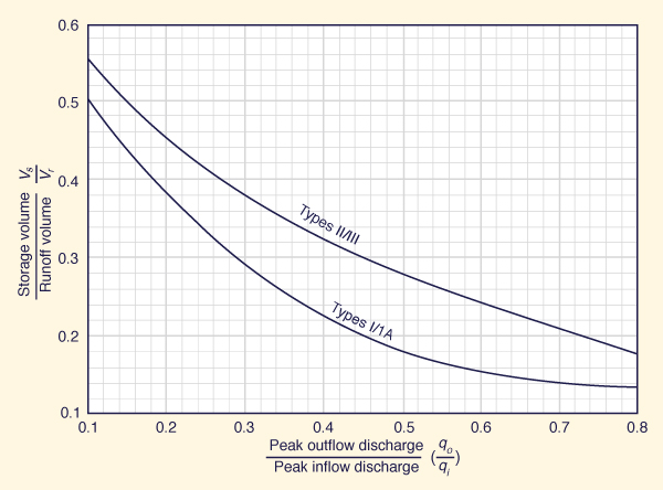
The TR-55 detention basin method is based on average storage and routing effects for many structures. The curves shown in Fig. 8-15 depend on the relationship between available storage, outflow device, inflow volume, and shape of the inflow hydrograph. When the required storage volume (Vs) is small, the shape of the outflow hydrograph is sensitive to the rate-of-rise of the inflow hydrograph. In this case, parameters such as rainfall volume, curve number, and time of concentration become especially significant. Conversely, when the required storage volume is large, the shape of the outflow hydrograph is little affected by the rate-of-rise of the outflow hydrograph. In this case, the outflow hydrograph is controlled by the hydraulics of the outflow device, and the procedure yields more consistent results [6].
The procedure is recommended for final design if an error in storage of 25 percent may be tolerated. The method may significantly overestimate the required storage capacity, because it is biased to prevent undersizing of outflow devices. Detailed hydrograph analysis and reservoir routing (Section 8.3) will generally result in reduced project costs.
Example 8-4.
A development is planned for a 30-ha catchment in Colorado and a detention basin is needed to reduce the impact of the development on downstream flood flows.
The existing concrete-lined channel has a capacity of 5 m3/s.
The planned development will produce a storm runoff depth of 85 mm and a peak discharge of 10 m3/s at the catchment outlet.
Size a detention basin to reduce the post-development peak flow to pre-development conditions.
The ratio of peak outflow to peak inflow, i.e., pre-development peak flow to unattenuated post-development
peak flow, is: Qo / Qi = 5/10 = 0.5.
From Fig. 8-15, for a Type II storm (Colorado): Vs / Vr = 0.277.
The storm runoff volume is: Vr = 300000 m2 × 0.085 m = 25500 m3.
Therefore, the detention basin storage volume is: Vs = 0.277 × 25500 = 7063.5 m3.
ONLINE CALCULATION.
Using ONLINE TR-55 DETENTION, the answer
is 7063.5 m3, which is the same as the hand calculation.
|
QUESTIONS
|
|
What is reservoir routing?
What is a linear reservoir?
What is the proportional or Sutro® spillway?
What is the differential equation of storage? What principle is it based on?
What is the xt plane?
Above what value of the storage constant K will one of the routing coefficients be negative?
Explain why in reservoir routing with uncontrolled outflow, the peak outflow occurs when inflow and outflow coincide.
Explain why there is no lag between inflow and outflow in reservoir routing.
What is the storage indication quantity?
What is an appropriate value of time interval to choose in reservoir routing?
What is surcharge storage?
Name three applications of reservoir routing.
What is a detention basin? When is it used?
PROBLEMS
|
|
Route the following inflow hydrograph through a linear reservoir:
Time (h) 0 1 2 3 4 5 6 7 8 9 10 Inflow (m3/s) 0 10 20 30 40 50 40 30 20 10 0 Assume baseflow = 0 m3/s, K = 3 h, Δt = 1 h.
Route the following triangular inflow hydrograph through a linear reservoir: peak inflow = 120 m3/s, baseflow = 0 m3/s, time-to-peak = 6 h, time base = 16 h, storage constant K = 2 h, and time interval Δt = 1 h.
Route the following inflow hydrograph through a linear reservoir.
Time (h) 0 1 2 3 4 5 6 7 8 9 10 11 12 Inflow (m3/s) 10 20 50 80 90 100 90 60 50 40 30 20 10 Assume baseflow = 10 m3/s, K = 4 h, Δt = 1 h.
Develop a spreadsheet to route a triangular inflow hydrograph through a linear reservoir. Inputs to the program are the following: peak inflow, baseflow, time-to-peak, time base, storage constant, and time interval. Test your work using Problem 8- 2.
Use the spreadsheet developed in Problem 8-4 to route the following inflow hydrograph: peak inflow = 750 m3/s, baseflow = 50 m3/s, time-to-peak = 3 h, time base = 8 h, storage constant
K = 1.5 h, time interval Δt = 0.5 h.Develop a spreadsheet to route an inflow hydrograph of arbitrary shape through a linear reservoir. Inputs are the following: inflow hydrograph ordinates, baseflow, reservoir storage constant, and time interval. Test your work using Problem 8-3.
Use the spreadsheet developed in Problem 8-6 to study the sensitivity of the outflow hydrograph to the chosen value of storage constant K. Use the following inflow hydrograph:
Time (h) 0 1 2 3 4 5 6 7 8 9 10 11 12 Inflow (m3/s) 0 10 30 50 80 100 90 60 40 30 20 10 0 Assume baseflow = 0 m3/s, and Δt = 1 h. Report calculated peak outflow and time-to-peak for (a) K = 1 h, (b) K = 2 h, (c) K = 3 h, and (d) K = 4 h. Verify your results using the online calculator ONLINE ROUTING01.
Using a spreadsheet, solve Problem 8-1 by the storage indication method. Verify with ONLINE ROUTING02.
Using a spreadsheet, solve Problem 8-2 by the storage indication method. Verify with ONLINE ROUTING02.
Using a spreadsheet, solve Problem 8-3 by the storage indication method. Verify with ONLINE ROUTING02.
Use ONLINE ROUTING03 to solve the following reservoir routing problem: emergency spillway width L = 15 m, rating coefficient Cd = 1.886, rating exponent y = 1.5, emergency spillway crest elevation = 730 m, dam crest elevation = 735 m, initial pool elevation = 730.5 m, baseflow = 10 m3/s. At spillway crest elevation, the reservoir storage is 3,000,000 m3, increasing linearly to 4,000,000 m3 at dam crest elevation. The inflow hydrograph is the following:
Time (h) 0 1 2 3 4 5 6 7 8 9 10 11 12 Inflow (m3/s) 10 30 70 150 210 250 170 110 70 50 30 20 10 Set Δt = 1 h. Report peak outflow, time-to-peak, maximum pool elevation, and effective freeboard.
Using the data of Problem 8-11, modify the volumetric characteristics of the reservoir to the following: storage at spillway crest elevation, 6,000,000 m3; storage at dam crest elevation, 8,000,000 m3. Run ONLINE ROUTING03 using Δt = 1 h. Report peak outflow, time-to-peak, maximum pool elevation, and effective freeboard. Compare with the results of Problem 8-11, explaining the differences.
Determine the actual freeboard for the following dam, reservoir, and flood conditions: dam crest elevation = 125 m; emergency spillway crest elevation = 120 m; coefficient of spillway rating Cd = 1.7; exponent of spillway rating y = 1.5; width of emergency spillway (rectangular cross section) L = 18 m.
Elevation-storage relation:
Elevation (m) 120 121 122 123 124 125 Storage (m3) 3,000,000 3,050,000 3,150,000 3,350,000 3,750,000 4,250,000 Inflow hydrograph to reservoir:
Time (h) 0 1 2 3 4 5 6 7 8 9 10 Inflow (m3/s) 0 10 15 30 55 85 105 125 150 135 110
Time (h) 11 12 13 14 15 16 17 18 19 20 21 Inflow (m3/s) 95 72 55 38 29 14 9 7 2 1 0 Assume the initial reservoir pool level at spillway crest. Use ONLINE ROUTING03.
Design the emergency spillway width L (to a 0.1 m accuracy) for the following dam, reservoir, and flood conditions: dam crest elevation = 483 m; emergency spillway crest elevation = 475 m; coefficient of spillway rating = 1.7; exponent of spillway rating = 1.5.
Elevation-storage relation:
Elevation (m) 475 477 479 481 483 Storage (m3) 5100,000 5300,000 5600,000 6400,000 7600,000 Inflow hydrograph to reservoir:
Time (h) 0 1 2 3 4 5 6 7 8 9 10 11 12 Inflow (m3/s) 0 10 30 50 90 150 250 350 280 210 190 170 130
Time (h) 13 14 15 16 17 18 19 20 21 22 23 24 Inflow (m3/s) 100 90 75 50 40 30 15 10 5 2 1 0 Assume minimum design freeboard = 3 m, and initial reservoir pool level at spillway crest. Use ONLINE ROUTING03.
A development is planned for a 85-acre watershed that outlets into an existing channel designed for present conditions. If the channel capacity is exceeded, damages will be substantial. The watershed is in the Type I storm distribution region. The present channel capacity is 150 cfs. The planned development will produce a storm runoff depth of 3 in. and a peak discharge of 320 cfs at the watershed outlet. Size a detention basin to reduce the post-development peak flow to pre-development conditions.
REFERENCES
|
|
Chow, V. T. (1964). Handbook of Applied Hydrology. New York: McGraw-Hill.
Garrison, J. M., J. Granju, and J. T. Price. (1969). "Unsteady Flow Simulation in Rivers and Reservoirs," Journal of the Hydraulics Division. ASCE, Vol. 95, No. HY9, September, pp. 1559-1576.
Laurenson, E. M. (1961). "Hydrograph Synthesis by Runoff Routing," Technical Report No. 66, Water Research Laboratory, University of New South Wales, Kensington, New South Wales, Australia.
Ponce, V. M., and D. B. Simons. (1977). "Shallow Wave Propagation in Open-channel Flow," Journal of the Hydraulics Division. ASCE, Vol. 103, No. HY12, December, pp. 1461-1476.
U.S. Army Corps of Engineers. (1959). "Reservoir Regulation," EM 1110-2-3600, Engineering and Design, Office of the Chief of Engineers, Washington, D.C., May 25, with changes of 26 December 1962.
USDA Natural Resources Conservation Service. (1986). "Urban Hydrology for Small Watersheds," Technical Release No. 55 (TR-55), Washington, D.C.
| http://engineeringhydrology.sdsu.edu |
|
221102 |