|
|
|
CHAPTER 3: HYDROLOGIC MEASUREMENTS |
|
"In river flow, the stochastic character of the collection of disturbances
causes a large-scale longitudinal mixing, which may be modeled as a diffusion equation containing a term of advection." Shoitiro Hayami (1951) |
|
This chapter is divided into five sections. Section 3.1 describes precipitation measurements and Section 3.2 deals with snowpack measurements. Section 3.3 describes evaporation and evapotranspiration measurements and Section 3.4 discusses infiltration and soil moisture measurements. Streamflow measurements are discussed in Section 3.5. |
3.1 PRECIPITATION
|
|
Introduction
Engineering hydrology is based on analysis and measurements. Measurements are necessary in order to complement and verify the analysis. Hydrologic measurements are usually performed in the field, using equipment and techniques specifically designed to measure a variable characterizing a certain phase of the hydrologic cycle. For instance, rainfall is measured with raingages, evaporation is measured with evaporation pans, and streamflow is measured using streamgaging techniques.
Measurements are closely related to hydrologic analysis. In some cases they are an integral part of it; in others, they serve to support it. For instance, statistical hydrology is not possible without measurements. In flood frequency analysis, a historical flow record is necessary in order to define the properties of the predictive equations. With parametric models, measurements aid in parameter estimation, increasing model reliability. Deterministic and conceptual models also benefit from hydrologic measurements.
Precipitation
Precipitation is measured with raingages. A raingage is an instrument that captures precipitation and measures its accumulated volume during a certain time period. The precipitation depth for the given period is equal to the accumulated volume divided by the collection area of the gage. The average precipitation intensity is equal to the precipitation depth divided by the length of the period.
Any receptacle that has vertical sides and is open to the air is a defacto raingage and can provide valuable information on accumulated rainfall during a storm. Two such measurements, however, are not directly comparable unless the receptacles are of the same size and shape and similarly exposed. To increase the utility of the measurements, it is necessary to use standard equipment and procedures.
Raingages can be of two types:
- Nonrecording, or
- Recording.
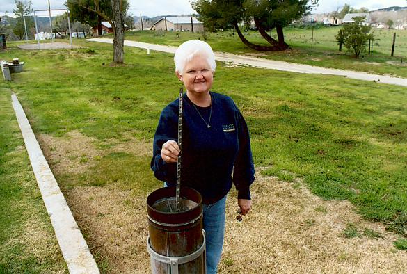
A nonrecording raingage measures the total rainfall depth accumulated during one time period,
usually
Fig. 3-1 Nonrecording raingage at the Campo Weather Station, San Diego County, California |
A recording raingage records the time it takes for rainfall depth accumulation. Therefore, it provides not only a measure of rainfall depth but also of rainfall intensity. The slope of the curve showing accumulated rainfall depth versus time is a measure of the instantaneous rainfall intensity. Recording rain gages rely on one of the following devices:
- A tipping bucket,
- A weighing mechanism, or
- A float chamber.
The tipping-bucket gage features a two-compartment receptacle (i.e., the bucket) pivoted on a knife edge. The device is calibrated so that when one of the compartments is full (with a fixed amount of rain) and the other is empty, the bucket overbalances and tips. At the start, rain is funneled into one of the compartments, which is positioned for filling. As rainfall continues to fill this first compartment, the second remains empty. When the first compartment is full, the bucket tips, emptying its contents into a reservoir and at the same time placing the second compartment in filling position. The tipping closes an electric circuit, which drives a pen that records on a strip chart affixed to a clock-driven revolving drum. Thus, each electrical contact representing a specific amount of rain is recorded. The alternate filling and emptying of the two compartments continues until rainfall ceases.
The tipping-bucket gage has a few disadvantages. During periods of intense rainfall, some of the rain may not be measured while the bucket is tipping. In addition, the record consists of a series of steps rather than being a smooth curve, and the gage is not suitable for measuring snow. Nevertheless, tipping-bucket gages are durable, simple to operate, and of good overall reliability.
A weighing gage has a device that weighs the rain or snow collected in a bucket. As it fills with precipitation, the bucket moves downward and its movement is transmitted to a pen on a strip-chart recorder. This type of gage is useful in cold climates where it is necessary to record both rainfall and snowfall. However, weighing gages have some disadvantages. Among them are wind action on the bucket, which produces erratic traces on the recording chart, and the overall lack of sensitivity of the measurement.
Float gages are essentially water-level gages. A float located inside a chamber is connected to a pen on a strip-chart recorder. The float rises as the collected rainwater enters the chamber, and the rise of the float is recorded on the chart. Some float gages are limited to the capacity of the chamber. Others are equipped with a self-starting siphoning device that empties the chamber when it becomes full and returns the pen to the zero position on the strip chart. The use of float gages is limited to nonfreezing ambient temperatures, although heaters and other similar devices have been used in an attempt to overcome the problem of freezing. Oil and mercury, which have freezing temperatures below that of water, have also been used inside the chamber. The siphoning action of the float gage can cause serious losses of rain during severe storms.
Errors in Measuring Precipitation Data
The water collected by a raingage is only a small sample of the precipitation that has fallen in a certain area. Whether this sample is representative of the average precipitation over the area remains to be determined by further analysis.
A series of rain gages located within a drainage area constitutes a raingage network. The density of the network is the number of rain gages per square kilometer (or square mile). The error of rainfall measurements can be investigated by studying the spatial averages computed from networks of different densities [1, 13, 23]. In general, sampling errors increase with an increase in rainfall depth. Conversely, sampling errors decrease with an increase in network density, storm duration, and catchment area.
An important question in engineering hydrology is whether errors in precipitation measurement can serve to compound the errors inherent in the use of rainfall-runoff simulation models. The answer to this question is elusive. Limited data by Johanson [11] indicates that the error variability in precipitation measurements is likely to be less than the error variability in model calibration. Calibration is the process by which model parameters are adjusted to match measured and simulated flows.
Precipitation Measurements Using Telemetry
Self-reporting rain gages (or rainfall sensors) have automatic data transmittal capabilities. These rain gages use automatic radio transmitters (telemeters) to broadcast rainfall measurements from a remote station to a central station in real time, i.e., during the storm event (Fig. 3-2). The advantage of a telemetric station is that it shortens the time that would otherwise be required to gather rainfall data. In certain cases, especially when speed of processing is of utmost importance, a network of rainfall sensors linked by telemetry may be the only practical means of collecting rainfall data. Applications of telemetric rainfall sensors are usually found in connection with operational hydrology and real-time flood forecasting.
Fig. 3-2 A telemetric weather station (Davis). |
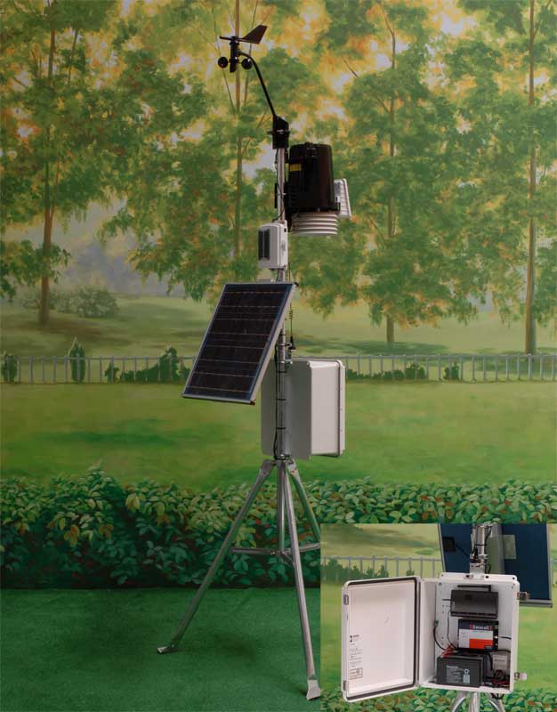
The link between the remote station and the central station is usually established by radio, telephone, or a combination of both. Where radio frequencies are scarce, telephone lines can be used to transmit the data. The remote rainfall station is interfaced to a telephone line either through a modem or an acoustic coupler. The latter enables the remote station to be called from any telephone, whether it is equipped with a modem or not.
Radio transmission may take the form of a very high frequency (VHF) or ultrahigh frequency (UHF) link for short distances, or high frequency (HF) for very long distances. VHF and UHF frequencies behave in a manner similar to light and, therefore, cannot travel far beyond the horizon. The best reception is obtained when the transmitting and receiving antennas are within line of sight of each other. With the use of high masts, a span of 40 km or more can be achieved. Transmitter power ranges from 5 W for short distances to 25 W for longer distances.
Very long distance transmissions require repeating stations at 30- to 60-km intervals, but these are expensive and difficult to maintain. An alternative is to use HF radio, by which great distances can be spanned through a series of reflections between ionosphere and ground. Normal transmissions have a span of a few hundred kilometers. These HF links, however, are subject to variations in signal strength and are susceptible to interference with other transmitters, making their use more difficult than VHF and UHF.
Another way to transmit data through radio waves is by the use of satellites. A remote station can transmit data to a satellite for retransmirtal to a ground receiving station. The radio link operates in the UHF range and requires only a few watts of power. To transmit data via a satellite, the station is linked to a commercially made data collection platform. This device stores the day's data in its solid state memory for transmission every 24 h, although hourly transmissions are also possible.
Precipitation Measurements Using Radar. Weather radar systems are a potentially powerful tool for measuring the temporal and spatial variability of rainstorms. A radar system operates by emitting a regular succession of pulses of electromagnetic radiation from its antenna. The pulses are on the order of 1 μs, and the system emits approximately 1000 of these pulses every second. Between pulses, the system's antenna becomes a receiver of the energy of the emitted pulses scattered by various targets. These returned signals are transformed into a visual display on the radar scope.
For spherical objects (e.g., raindrops), the power received can be expressed as follows:
|
K Σ n D 6
P = __________ λ 4R 2 | (3-1) |
in which P = power received, n = number of drops, D = diameter of drops, λ = wavelength of the radiation, R = distance (range) from the radar, and K = a factor that depends on the power of the transmitted signal, antenna size and shape, and properties of the scattering particles.
Weather radars have wavelengths in the range of 3 to 10 cm. Following Eq. 3-1, a 3-cm radar returns about 120 times as much power as that returned by a 10-cm radar. Hence a 3-cm radar can detect weak targets such as the small droplets associated with very light rain, whereas a 10-cm radar can be used to sense much heavier rains.
Attenuation, caused by absorption and scattering by clouds and precipitation, can also affect the performance of the radar. Attenuation is a function of radar wavelength, being greater for shorter wavelengths.
The reduction in power received P with distance R (range) is a constant for a given system and can be adjusted to make distant targets show the same brightness as closer targets of similar character. Since power P is proportional to the sixth power of the drop diameter D, radars in the 3- to 10-cm wavelength size can easily sense rainsize droplets and not sense other size particles at all. A 10-cm radar is used for detecting highly intensive storms, which are likely to produce extreme floods. For light rains or snow sensing, a shorter wavelength radar is preferable.
The radar reflectivity (ΣnD 6) can be empirically related to precipitation intensity as follows:
| Z = A I B | (3-1) |
in which Z = radar reflectivity; I = precipitation intensity; and A and B are empirical constants. The values of A and B depend upon the type of precipitation being observed. Many values have been specified; those most often used are A = 200 and B = 1.6 [4].
Several types of error are possible when using radar to sense precipitation. For instance, the radar beam can overshoot shallow precipitation at long ranges, missing the target. Another source of error is the presence of low level evaporation beneath the radar beam, as well as several other meteorological factors [7]. Uncertainties in radar sensing of precipitation can be resolved by calibrating the system with a raingage. This is usually accomplished by fixing exponent A (in Eq. 3-2) at a certain value (for instance B = 1.6), and using raingage data to derive a value of coefficient A.
3.2 SNOWPACK
|
|
Measurements of snow include both newly fallen snow and snow accumulation, i.e., snowpack. Snowpack measurements are expressed in terms of water equivalent, i.e., the depth of water that is obtained after melting a certain depth of snowpack. Water equivalent is a measure of the amount of water remaining in storage in the snowpack. Water-equivalent data are useful in water yield forecasts, since they integrate in one measurement both snowfall and snowmelt.
As with rainfall measurements, snowfall or its water equivalent must be measured by sampling at several points and averaging point values to obtain a representative value of the snowpack. A simple method for measuring snowfall is to use a snowboard. The snowboard is placed on the ground or on old snow surface to permit the accumulation of new snow on top of it. An inverted raingage cylinder is used to isolate a core of the new snow, which is then melted and measured in the same way as rainfall. By measuring each fall of snow in this manner and replacing the clean board ready to receive fresh snowfalls, accumulated total snowfall throughout the season may be known at any time. Such measurements are fairly reliable, provided that they are taken soon after each snowfall and that the snow on the board has not been subjected to drifting, melting, or evaporation.
The density of a snow sample is the ratio of the volume of melt water to the initial volume of the sample, expressed as a percentage. Snow density in the typical snowpack varies widely, both within the vertical structure of the snowpack and with time.
Snow stakes are often used to measure snow accumulation. Water equivalent of the snowpack can be determined from depth measurements by using known densities of snow, obtained under similar environmental conditions. Snow stakes are also used where it is impractical to obtain water equivalents by direct sampling.
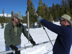
Direct sampling of water equivalent is accomplished by the use of snow samplers. The Mount Rose sampler is commonly used in the United States. It consists of a tube fitted with a cutter on one edge. The tube has an inside diameter of 1.485 in., so that a core weighing 1 oz is equivalent to 1 in. of water. Sampling consists of pushing the tube vertically into the snow to full snow depth, withdrawing the tube with the snow content, and weighing the contents (Fig. 3-3).
Fig. 3-3 Weighing a Mount Rose sampler (National Park Service). |
Snow Courses
When performing snow measurements, common practice is to sample water equivalent at a number of points along an established line called a snow course. Snow courses are selected with the objective of obtaining representative data from a given area. The number of snow courses varies, depending on terrain features and meteorological characteristics. Site selection considers the following aspects:
- Meteorological conditions related to storm experience,
- Position with respect to large-scale topographic features,
- Position with regard to local environmental features, such as wind, exposure, orientation, and ground slope, and
- Site conditions, including local drainage and presence of brush or rocks.
In addition, snow courses are positioned so that they are representative not only of snowfall but also of snowmelt.
The number of sample points varies depending upon the consistency in the spatial distribution of snow. Sample points should avoid the effect of trees, boulders, and other obstructions. If there is little protection from the wind, sample points are spread over a wide area to average out variations due to drifting. In general, five snow-course sample points are adequate for well-positioned snow courses that have a minimum of irregularities caused by drifting or wind erosion and a smooth ground surface clear of obstructions. When conditions are less than ideal, additional snow-course points are required for adequate sampling of the water equivalent.
Radioisotope Snow Measurements
Specially designed radioisotope snow gages with telemetering capabilities are used to measure the water equivalent of snowpack at remote, unattended sites. The equipment measures water equivalent by correlating it with the attenuation of a gamma ray emission (cobalt 60) as it travels through the snow from source to detector. The original equipment had the source positioned at ground level, with the detector 15 ft above it [28]. Later models were reversed to minimize temperature effects on the detector, with the detector positioned at ground level and the source 15 ft above it [16]. Recalibration of radioisotope snow equipment at regular intervals is necessary to guarantee the accuracy of the measurement.
Profiling radioactive snow gages are used to determine the variation of water equivalent within the snowpack depth [21]. These gages consist of a gamma photon source and detector, which are moved synchronously through vertical tubes located about 60 cm apart in the snowpack. The gages are used for measuring temporal and spatial variations in snowpack properties.
Determination of Catchment Water Equivalent
Point values from all snow courses representative of an area are used to determine catchment water equivalent. The relationship between catchment water equivalent and point values is dependent upon fhe location of the snow courses. When snow courses are distributed equally throughout the range of elevations, an arithmetic average of point values usually provides a satisfactory value of catchment water equivalent. Refinements can be obtained by weighing data from each snow course in proportion to the percentage of catchment area covered by it.
Elevation is an important factor in converting point measurements into catchment water equivalent. Generally, snow courses tend to be concentrated at higher elevations, and therefore an arithmetic average is not appropriate. An alternative is to develop a snow chart, a plot showing the variation of water equivalent with elevation. This chart is used together with the catchment's area-elevation curve (i.e., the hypsometric curve, Section 2.3). The catchment's elevation difference is divided into several equal increments. For each elevation increment, a subarea is obtained from the area-elevation curve, and a corresponding water equivalent is obtained from the snow chart. A water equivalent value representative of the entire catchment can be obtained by weighing the individual water equivalents in proportion to their respective subareas.
Sources of Snow Survey Data
The Federal-State-Private Cooperative Snow Survey System publishes snow survey data on a regular basis.
The system is coordinated by the Soil Conservation Service, with jurisdiction in the Western United States.
The State of California, however, maintains its own snow survey system, administered by its Department of
Water Resources. In the Eastern United States, several federal, state, and private agencies perform snow
surveys. These are used for various purposes, including fish and wildlife management, recreational uses,
and highway maintenance. Federal agencies collecting snow survey data are the National Weather Service and the U.S. Geological Survey.
3.3 EVAPORATION AND EVAPOTRANSPIRATION
|
|
A practical way to measure evaporation directly is by the use of an evaporation pan. The pan exposes a free water surface to the air, and the evaporation rate is determined by measuring the water loss during one time period, usually 1 day. The evaporation rate measured by the pan, however, is generally not the same as that of a lake or reservoir exposed to similar meteorological conditions.
The difference is attributed to the pan installation and exposure. For example, a pan installed on supports above the ground surface is subject to extra radiation on the sides. On the other hand, a buried pan is subject to appreciable heat exchange between it and the surrounding soil. These and other factors contribute to make the overall heat balance for the pan a complex phenomenon.
The factors responsible for the discrepancy usually combine to produce a pan measurement that is greater than the actual lake or reservoir evaporation. Therefore, a correction factor is applied to the pan evaporation measurement in order to arrive at the actual value of lake or reservoir evaporation. This correction factor is referred to as the pan coefficient.
NWS Class A Pan
The National Weather Service Class A pan is the most widely used evaporation pan in the United States. This pan has been recommended as a standard for evaporation measurements by the World Meteorological Organization.
The Class A pan is made of unpainted galvanized iron, has a diameter of 122 cm (4 ft) and a height of 25.4 cm (10 in.) and is mounted about 15 cm (6 in.) above the ground on supports which permit a free flow of air around and under the pan (Fig. 3- 4). Water loss is determined by daily measurements of water level using a micrometer hook gage installed in a stilling well set inside the pan. The pan is initially filled to a height of 20 cm (8 in.) and is refilled when the water level has fallen below 17.5 cm (7 in.). Daily evaporation is computed as the difference between two successive observations, corrected to account for any intervening precipitation (measured in a nearby gage). An alternate procedure is to add a measured amount of water daily to bring the water level in the pan up to a fixed point in the stilling well. This procedure permits a more accurate measurement of water loss and assures that the pan has the proper water level at all times.
Fig. 3-4 NWS Class A evaporation pan (University of Iowa). |
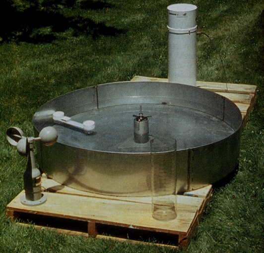
Because of interception of solar radiation by the sides, the Class A pan, like other similarly exposed pans, usually exaggerates the actual lake or reservoir evaporation. Therefore, its pan coefficient is less than 1, with an annual average of approximately 0.7 (see Table 2-8).
Little is known about the spatial variability of evaporation. However, it seems likely that it is not as large as that of precipitation. If this is the case, a network of much lesser density would be required for a correct assessment of evaporation. For general purpose and preliminary evaporation estimates, a density of one station per 5000 km2 appears to be sufficient [14].
Evapotranspirometers
Evapotranspirometers are instruments designed to measure potential evapotranspiration (PET). An evapotranspirometer consists of a central tank and at least two other watertight soil tanks. The soil tanks are open to the air above them and are connected through underground pipes to collecting cans located in the central tank. The soil tanks support a continuous vegetative cover, such as grass. Water can enter the soil tanks only from above, either as natural or artificial precipitation, and can leave the tanks only through the bottom pipes directly into the collecting cans in the central tank. During one time period, the difference between the amount of water entering each soil tank and the amount of water accumulated in the respective collecting can is the water lost to evapotranspiration, provided the proper allowance is made for changes in moisture storage in the soil tank. If the soil moisture in the tank is maintained at field capacity, the measured difference represents PET.
Evapotranspirometer measurements are made daily. The soil tanks are sprinkled with a known quantity of water, which varies depending on the time of the year (season) and on the amount of precipitation that fell on the previous day. To minimize soil leaching, the water that percolated the day before is mixed with the irrigation water. Evapotranspiration depth is equal to precipitation depth plus irrigation depth minus percolation depth. Soil moisture, however, rarely remains constant from day to day. For instance, it increases greatly during and immediately after precipitation. Therefore, on rainy days, the measurement usually indicates a high PET value, whereas the following day it indicates a low and perhaps even a negative PET value. Only during a prolonged period with no precipitation would the measurements give an accurate indication of the day-to-day variations of PET. However, long-term, i.e., monthly or seasonal, values are likely to be fairly good representations of PET.
Lysimeters
Lysimeters are instruments designed to measure actual evapotranspiration. Actual evapotranspiration is much more difficult to measure than potential evapotranspiration. During the summer months when soil moisture may be considerably depleted, actual rates of evapotranspiration fall well below the potential rate. The actual rate is determined not only by climatic factors but also by the ability of the plant to extract water from the soil and by the speed of movement of soil moisture to the plant roots.
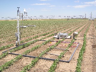
A properly constructed Iysimeter must be representative of the surrounding area. Vegetation cover, surface conditions, soil structure, porosity, stratification, and water-flow relationships (infiltration, permeability, and capillarity) must remain as true to the prototype as possible (Fig. 3-5). Ideal conditions are rarely obtained, particularly when actual evapotranspiration is markedly less than potential evapotranspiration.
Exact duplication within the soil tanks of the natural conditions usually requires that the size of a lysimeter tank be greater than that of an evapotranspirometer. The larger the tanks, the less the influence of edge effects and the greater the likelihood that the root systems in the tank will simulate natural conditions. Inevitably, the greater the tanks, the heavier they become, and the more cumbersome and difficult they are to handle. For instance, the set of weighing monolith lysimeters at Coshocton, Ohio [9], are 2.4 m (8 ft) deep and 3.1 m (10 ft) in diameter. Other Iysimeter experiments have been reported in the literature; see, for example, [15].
Fig. 3-5 A field lysimeter (Agricultural Research Service). |
3.4 INFILTRATION AND SOIL MOISTURE
|
|
Infiltration rates vary greatly, both in time and space. Therefore, care should be taken to ensure that a measurement or a series of measurements are representative of the area under study. In practice, infiltration rates are determined either by the use of infiltrometers or by the analysis of rainfall-runoff data from natural catchments.
Infiltrometers
Infiltrometers are instruments designed to measure the rate at which water is absorbed by the soil surface enclosed within a small, clearly defined area. There are two types of infiltrometers:
- Flooding, and
- Sprinkler.
A flooding infiltrometer consists of two concentric metal rings that are inserted a distance of 2 to 5 cm into the ground (Fig. 3-6). The rate at which water must be applied to the inner ring to maintain a constant head of 0.5 cm is taken as a measure of infiltration rate. In order to prevent the water from spreading laterally below the ground surface, the same head of water is maintained in the annular space between the rings.
Fig. 3-6 A flooding infiltrometer. |
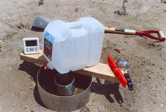
Many factors contribute to make the infiltration rate measured with a flooding infiltrometer different from actual infiltration rate. For one thing, the insertion of the rings disturbs the soil immediately around them, leading to an increase in infiltration rate. Differences in head between inner and annular spaces are also likely to cause divergence. Moreover, the flooding condition is not representative of actual conditions. Usually, all these factors combine to produce a high estimate of infiltration rate from a flooding infiltrometer. In addition, a large number of these tests are required for assessment of the spatial variability of infiltration.
A sprinkler infiltrometer is designed to avoid some of the pitfalls of the flooding infiltrometer. In the sprinkler infiltrometer, a simulated rainfall condition is applied over a small plot by using sprinklers. A common plot in use is the F plot, which is 1.8 m wide and 3.6 m long. In the F plot, large drops are applied to the plot and surrounding areas from two rows of special nozzles mounted along each long side of the plot. These nozzles direct their spray upward and slightly inward to cover the plot with relatively uniform rainfall intensities of about 4.5, 9.0, and 13.5 cm/ h, depending on how many sets of nozzles are used. The drops reach a height of 2 m above the plot surface and are therefore able to produce erosion and surface conditions resembling those of natural rain [17]. The simulated rainfall is continued for as long as necessary to attain an equilibrium runoff condition at the plot outlet. Average infiltration rate is calculated as the difference between the constant rainfall rate and the constant (i.e., equilibrium) runoff rate.
Due to the spatial and temporal variability of infiltration, field measurements can provide only qualitative information, best suited for comparative studies. Quantitative estimates that are representative of actual conditions are more likely to be obtained from methods based on rainfall-runoff analysis.
Infiltration Rates from Rainfall-Runoff Data
The use of rainfall-runoff data to determine infiltration rates represents an extension of the sprinkler infiltrometer technique. For a storm with a single runoff peak, the procedure resembles that of the calculation of a φ-index (Section 2.2). The rainfall hyetograph is integrated to calculate the total rainfall volume. Likewise, the runoff hydrograph is integrated to calculate the runoff volume. The infiltration volume is obtained by subtracting runoff volume from rainfall volume. The average infiltration rate for the given storm is obtained by dividing inftltration volume by rainfall duration.
The procedure can be extended to complex storms consisting of several substorms and related runoff peaks. First, it is necessary to use hydrograph separation or similar techniques to isolate the various sub storms and their corresponding hydrographs (Sections 5.2 and 11.5). By calculating sets of rainfall and runoff volumes for each substorm, a measure of how the infiltration rate varies from one substorm to the next can be obtained. The procedure works best in cases where the hydrographs can be readily separated, particularly for upland catchments. The procedure is also recommended for cases where interception and surface storage are negligible as compared to infiltration. Interception can be assumed to be insignificant for highly intensive storms, whereas surface storage is likely to be small in catchments with high relief. When used judiciously, this type of analysis can provide a reliable means of determining infiltration rates.
A factor to take into account when using rainfall-runoff analysis to determine infiltration rates is the effect of long-term storage. For large basins, the time elapsed between rainfall and runoff may be so great that it may be practically impossible to determine the amount of runoff produced by a storm event within a reasonable length of time. In practice, this limits infiltration analysis based on rainfall-runoff data to basins with negligible long-term storage.
Measurements of Soil Moisture
Two levels of soil moisture are used in engineering hydrology:
- Field capacity, and
- Permanent wilting point.
The field capacity is the maximum amount of moisture that the soil structure can hold against the force of gravity. It characterizes the upper level of moisture above which additional infiltration will tend to pass rather rapidly through the soil. The permanent wilting point is the soil moisture content at which permanent wilting of plants starts to occur.
Soil moisture can be measured directly or indirectly. The direct measurement involves the determination of the weight loss from several oven-dried field samples. Each sample is weighed before and after being dried at a temperature of 105°C. The moisture content is the ratio of the weight of water loss to the weight of the dry soil, as a percentage. These measurements, however, are time consuming and do not provide a record of the continuous change of soil moisture with time.
Indirect measurements of soil moisture involve the use of tensiometers to measure the suction force with which water is held in moist soil. The instrument consists of a tube full of water, with a porous cup at the bottom and a stopper on top. The tube is connected to a mercury manometer or vacuum gage. When the tube is inserted into the soil, water moves through the porous cup to the surrounding soil, causing a pressure drop to register in the manometer. The drier the soil, the greater the amount of water leaving the tube and, consequently, the greater the pressure decrease. Tensiometer tests can be performed in situ, but their application is restricted within a limited range of soil moisture [18, 19].
The neutron probe is a device used for indirect measurement of soil moisture content in the field [12, 24]. The method is based on the fact that fast neutrons are scattered and slowed down when they collide with the protons of hydrogen atoms. The probe consists of a fast neutron source and a slow neutron counter, which registers a high count when the soil moisture is high and a low count when the soil moisture is low. A calibration curve relates the neutron count to the moisture content of the soil. A clear advantage of the neutron probe is the speed of measurement; however, a disadvantage is that with the neutron probe it may be difficult to ascertain changes of soil moisture with depth.
The water balance method is another indirect way of determining soil moisture. The method is based on the assumption that soil moisture can be represented as the difference between precipitation (input) and evapotranspiration (output). Thus, moisture content can be evaluated directly from readily available precipitation and evapotranspiration data. When rainfall exceeds evapotranspiration, the soil moisture increases; conversely, when evapotranspiration exceeds rainfall, the soil moisture decreases. The water balance, however, must include the change in evapotranspiration with moisture availability. When soil moisture is high, evapotranspiration can take place at the potential rate; when soil moisture is low, the actual evapotranspiration rate is much lower than the potential rate. Thus, to use this method it is necessary to relate actual evapotranspiration to soil moisture. When sufficient data are available, this method can provide useful and accurate results [26, 27].
3.5 STREAMFLOW
|
|
The discharge at a given location along a stream can be evaluated in two ways: (1) either by measuring the stage and using a known rating to obtain the discharge from it, or (2) by directly measuring the cross-sectional flow area and mean velocity of the stream. The point along the stream where the measurements are made is called the gaging site or gaging station. The measurement of discharge and stage is referred to as stream gaging.
The development of a good rating curve is crucial to the accurate determination of discharge from stage (Fig. 3-7). The quality of the rating is evaluated in terms of its stability and permanence. A stable rating remains constant in time, i.e., the effects of flow nonuniformity, unsteadiness, or erosion and sedimentation are negligible. A permanent rating is one that is not likely to be disturbed by human activities.
Fig. 3-7 Rating curve for Mississippi River at Anoka, MN (National Weather Service). |
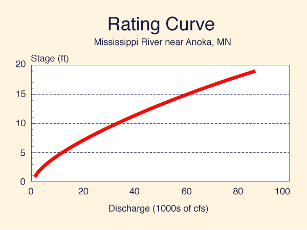
A gaging site should be located at a point along the stream where there is a high correlation between stage and discharge. Stated in other terms, the stage-discharge rating should be close to being single-valued, i.e., featuring a one-to-one correspondence between stage and discharge. Either section or channel control is necessary for the rating to be single-valued.
A rapid or fall located immediately downstream of a gaging site forces critical flow through it, providing a section control. In the absence of a natural section control, an artificial control, for instance, a concrete weir, can be built to force the rating to become single-valued. This type of control is very stable under low and average flow conditions.
A long downstream channel of relatively uniform cross-sectional shape, constant slope, and bottom friction provides a channel control. However, a gaging site relying on channel control requires periodic recalibration to check its stability. To improve channel control, the gaging site should be located far from downstream backwater effects caused by reservoirs, large river confluences, or tides.
Stage Measurements
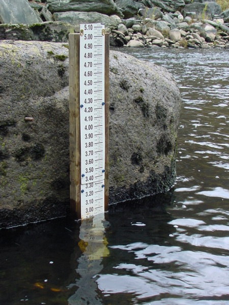
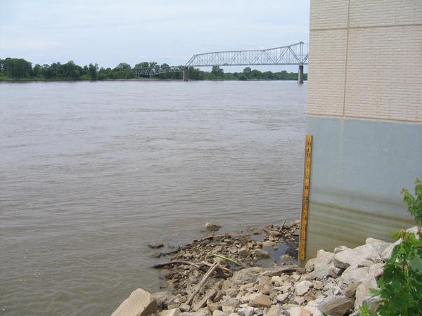
Manual Gages. The simplest type of manual gage is the vertical staff gage. This is a scale reading to centimeters (or tenths of a foot), which is vertically attached to a fixed feature such as a bridge pier or a pile (Fig. 3-8). The scale must be positioned so that all possible water levels can be read promptly and accurately. Where this is not feasible, several sectional staff gages are placed in such a way that one of them is always accesible for measurement (Fig. 3-9).
Fig. 3-8 A staff gage (Massachussets Department of Fish and Game). |
|
|
|
Another type of manual gage is the wire gage. Wire gages consist of a reel holding a length of light cable with a weight affixed to the end of the cable. The reel is mounted in a fixed position-for instance, on a bridge span-and the water level is measured by unreeling the cable until the weight touches the water surface. Each revolution of the reel unwinds a specific length of cable, permitting the calculation of the distance to the water surface.
Manual gages are used where stages do not vary greatly from one measurement to the next. They are impractical in small or flashy streams, where substantial changes in stage may occur between readings.
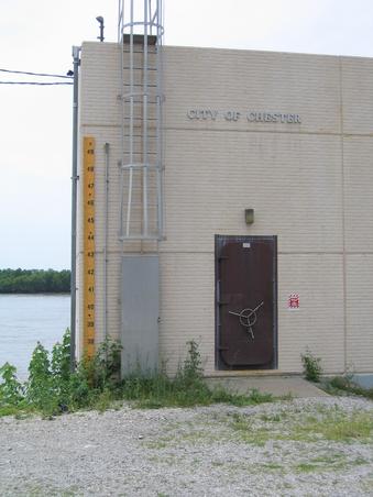
Recording Gages. A recording gage measures stages continuously and records them on a strip chart. The mechanism of a recording gage is usually either float-actuated or pressure-actuated. In the float-actuated recorder, a pen recording the water level on a strip chart is actuated by a float on the surface of the water. The recorder and float are housed in a suitable enclosure on top of a stilling well connected to the stream by two intake pipes (two pipes are used in case one of them becomes clogged). The stilling well protects the float from debris and ice and dampens the effect of wave action. This type of gage is commonly used for continuous measurements of water levels in rivers and lakes.
The pressure-actuated recorder eliminates the need for a stilling well. The sensing element of the recorder is a diaphragm, which is submerged in the stream. The changing water level produces a change in pressure on the diaphragm, which is transmitted to the recorder. Another type of pressure-actuated recorder is the bubble gage, developed by the U.S. Geological Survey [3]. The bubble gage consists of a specially designed servomanometer, gas-purge system, and recorder. Nitrogen fed through a tube bubbles freely into the stream through an orifice positioned at a fixed location below the water surface. The pressure in the tube, equal to that of the piezometric head above the orifice, is transmitted to the servomanometer, which converts changes in pressure in the gas-purge system into pen movements on a strip-chart recorder. In this way, a continuous record of stage is obtained.
Telemetric Gages. Gages with automatic data transmittal capabilities are called self-reporting gages, or stage sensors. These instruments use telemeters to broadcast stage measurements in real time, from a stream-gaging location to a central site. This type of gage is ideally suited for applications where speed of processing is of utmost importance, e.g., for operational hydrology or real-time flood forecasting.
Self-reporting gages are of the float-actuated or pressure-actuated type. The float-actuated type is used in stream and lake installations where a concrete abutment (e.g., a bridge pier) is already in place and where sediment loading is minimal. A typical station consists of a top section, which houses a transmitter and float-type water-level sensor, a stilling well with antenna mounting bracket. antenna cable, and connectors.
Bubble-type water-level sensors are used in applications where a stilling well is either impractical or too expensive and where the stream carries a heavy sediment load. In a typical installation, the bubbler orifice is anchored in the stream bed, and a plastic tube connects this orifice to a dry air or dry nitrogen supply and to a fluid manometer measuring assembly. Changes in river stage cause changes in piezometric head at the bubbler orifice. These changes in pressure are recorded by the manometer assembly. Data are transmitted automatically to a central station for further processing.
Other self-reporting stage sensors use a solid-state pressure transducer to sense pressure changes. They are used for measuring river stages where installation of a standpipe and stilling well is not feasible and where a highly sensitive device is not required. This type of sensor continues to provide readings even if a small amount of sediment builds up around the orifice.
Discharge Measurements
A discharge measurement at a stream cross section requires the determination of flow area and mean velocity for a given stage. The cross section should be perpendicular to the flow, and mean velocity should be based on a sufficient number of velocity measurements across the section.
In a typical stream-gaging procedure, each of several depth soundings, usually 20 to 30, defines the position of a vertical (Fig. 3-10). Each depth sounding is associated with a partial section of the stream. A partial section is a rectangle of depth equal to the sounding and of width equal to half the difference of the distances to adjacent verticals. At each vertical, the following observations are made:
- The flow depth, and
- The velocity as measured by a current meter at one or two points along the vertical.
Fig. 3-10 Streamgaging procedure. |
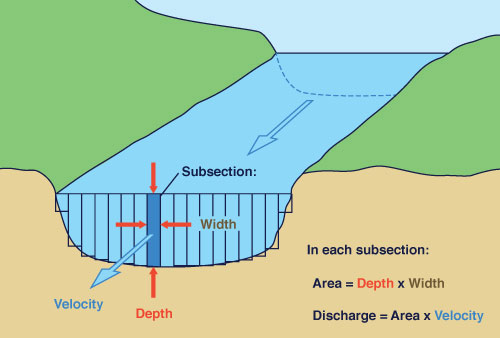
In the two-point method, the current meter is positioned at 0.2 and 0.8 of the flow depth. In the one point method, the current meter is positioned at 0.6 of the flow depth, measured from the water surface. The average of the velocities at 0.2 and 0.8 depth or the single velocity at 0.6 depth is taken as the mean velocity in the vertical. Where a two-point measurement is impractical (e.g., in very shallow streams), the one-point method is recommended.
For each partial section, the discharge is calculated as:
| q = v a | (3-3) |
in which q = discharge, v = mean velocity, and a = flow area. The total stream discharge Q is the sum of the discharges of each partial section.
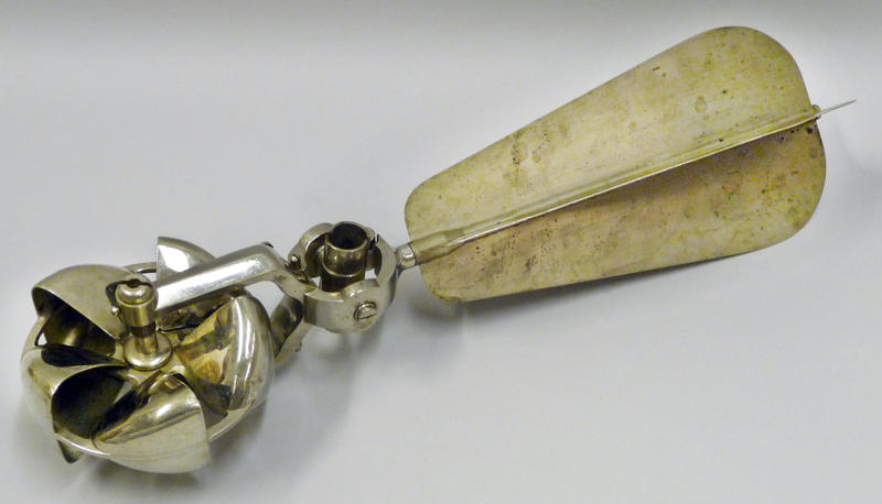
Current Meters. Current meters measure flow velocity by counting the number of revolutions per second of the meter assembly. The rotation can be around a vertical axis, leading to the cup meter, or around a horizontal axis, leading to the propeller meter.
Cup meters are widely used in the United States. The most common type of cup meter is the Price current meter, which has six cups mounted on a vertical axis (Fig. 3-11). The flow velocity is proportional to the angular velocity of the meter rotor. The flow velocity is determined by counting the number of revolutions per second of the rotor and consulting the meter calibration table.
Fig. 3-11 Price current meter. |
Calibration of a current meter is performed in a rating station, which has a reinforced concrete basin 20 m long, 1.8 m deep, and 1.8 m wide. On top of the vertical side walls of the basin and extending along its entire length are steel rails designed to carry an electrically driven rating car. Generally, the basin is full with still water. To calibrate the current meter, it is affixed to the rating car and positioned below the still water surface. The rating car is displaced at constant speed across the length of the basin. Paired observations of the velocity of the car versus the number of revolutions per second of the meter rotor lead to the rating expressed as:
| V = K N + C | (3-4) |
in which V = flow velocity as measured by the current meter; N = number of revolutions per second of the rotor assembly; and K and C are calibration constants [22].
Older current meters required periodic recalibration in order to minimize errors in velocity measurement due to wear or accidental damage. More recent models, however, have cups made of plastic and are so much alike that one rating can be used for several meters.
Price current meters types AA and A are used for two-point velocity measurements in streams with flow depths above 0.75 m and for one-point measurements in streams with depths ranging from 0.45 to 0.75 m. The dwarf (or pigmy) current meter is used for one-point measurements in shallow streams or laboratory flumes with depths in the range 0.10 to 0.45 m.
Current meter Measurements. Techniques for measuring stream velocity with a current meter vary with stream size. If the stream is wadable, the meter is affixed to a graduated depth rod. If the stream is too deep to wade, the meter is suspended on a cable and is held in the water with a sounding weight . The weights are made of various sizes, from 6.8 kg to 135 kg. Measurements using cable suspension are made from bridges, cableways, or boats (Fig. 3-12). For the heavier sounding weights or when using a boat, a sounding reel may be required.
Fig. 3-12 USGS streamgaging station, Campo Creek at Campo Road, |
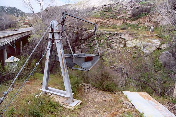
The current meter is affixed to a rod on top of the sounding weight. Soundings are made by setting the meter at the water surface and lowering it until the sounding weight rests on the stream bed. Velocity measurements are made either by the two-point or the one-point method. The size of the sounding weight is a function of the depth and swiftness of the stream. If the velocity of the stream is too high for the weight, the latter can drift downstream and greatly exaggerate the flow depth. In this case, it is necessary to reduce the measured depth to correct for downstream drift [5].
Chemical Methods for Measuring Velocity. Several chemical methods have been developed to measure stream velocity. They are normally used in cases where it is impractical to use current meters. Such is the case for shallow streams, very large rivers, or tidal flow. These methods can be grouped into
- Tracer, and
- Dilution methods.
A tracer is a substance that is not normally present in the stream and that is not likely to be lost by chemical reaction with other substances. Salt, fluorescein dye, and radioactive materials are commonly used as tracers. Small quantities of the tracer are injected into the stream at a source, and the time of travel to one or more downstream points is monitored.
When salt is used as a tracer, it is introduced at several points across a section. Electrodes are mounted at the two ends of a uniform reach beginning a short distance downstream from the salt source. These electrodes are connected to a recording galvanometer and are used to monitor the passage of the salt solution. The velocity of the stream is the length of the reach divided by the time that it takes the bulk of the salt solution to travel through the reach.
An expedient measurement of velocity can be obtained by timing the travel of floats. A surface float travels with a speed that is about 1.2 times the mean velocity. Floats extending well below the surface usually travel with a speed close to the mean velocity.
In the dilution method, a concentrated solution of a substance is introduced at a constant rate at a source point. Further downstream, after complete mixing has taken place, the flow is sampled to determine the equilibrium concentration of the mixture. A mass balance of flow and substance leads to the following equation:
| Cs Qs = Ce ( Q + Qe ) | (3-5) |
in which Cs = concentration of the substance solution at the source; Ce = equilibrium concentration of mixture at the sampling point; Qs = rate of inflow of substance solution at the source; and Q = stream discharge. Solving for Q from Eq. 3-5 leads to:
|
Cs Q = ( ___ - 1 ) Qs Ce | (3-6) |
The dilution method is particularly useful for very turbulent flows, which can provide complete mixing within a relatively short distance. It is also applicable when the cross section is so rough that alternative methods are unfeasible. The method requires the assurance of complete mixing and an accurate determination of equilibrium concentration of the mixture.
Physical Methods for Measuring Velocity.
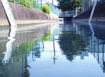
The ultrasonic and electromagnetic flowmeters are examples of physical devices to measure flow velocity. In the ultrasonic method, two sonic pulses are emitted and received, each at opposite banks of the river. The instruments are not located directly across from each other on the banks but rather on a diagonal line, making a 45° angle with the flow direction (Fig. 3-13). Therefore, one of the pulses travels with the current and the other against it. The difference in travel time between the two pulses is related to the longitudinal flow velocity. The method is applicable to large rivers where current metering or other direct techniques are not feasible. Its accuracy is claimed to be within 2 percent [10, 20].
Fig. 3-13 Setup of ultrasonic flow meter (JFE Advantech). |
The electromagnetic flowmeter is based on the fact that a conductor moving in an electromagnetic field generates a current within it. The river flow is a conductor cutting through the vertical component of the earth's magnetic field. The current can be measured by two electrodes, which are set at right angles to flow and magnetic field directions, respectively. The devices are applicable to measurement of tidal velocities, preferably in large rivers [2].
Indirect Determination of Peak Discharge: The Slope-Area Method
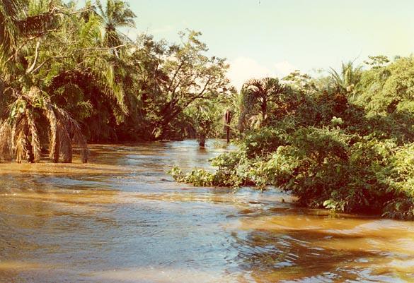
The high stages and swift currents that prevail during floods combine to increase the risk of accident and bodily harm (Fig. 3-14). Therefore, it is generally not possible to measure discharge during the passage of a flood. An estimate of peak discharge can be obtained indirectly by the use of open channel flow formulas. This is the basis of the slope-area method.
Fig. 3-14 Flood stage on the Chane river, Bolivia, on January 19, 1990. |
To apply the slope-area method for a given river reach, the following data are required:
The reach length,
The fall, i.e., the mean change in water surface elevation through the reach,
The flow area, wetted perimeter, and velocity head coefficients at upstream and downstream cross sections, and
The average value of Manning n for the reach [6].
The following guidelines are used in selecting a suitable reach:
- High-water marks should be readily recognizable,
The reach should be sufficiently long so that fall can be measured accurately,
The cross-sectional shape and channel dimensions should be relatively constant,
The reach should be relatively straight, although a contracting reach is preferred over an expanding reach, and
Bridges, channel bends, waterfalls, and other features causing flow non uniformity should be avoided.
The accuracy of the slope-area method improves as the reach length increases. A suitable reach should satisfy one or more of the following criteria:
The ratio of reach length to hydraulic depth should be greater than 75,
The fall should be greater than or equal to 0.15 m, and
The fall should be greater than either of the velocity heads computed at the upstream and downstream cross sections [8].
The procedure consists of the following steps:
Calculate conveyance K at upstream and downstream sections:
1
Ku = ( __ ) Au Ru 2/3
n
(3-7a) 1
Kd = ( __ ) Ad Rd 2/3
n
(3-7b) in which K = conveyance; A = flow area; R = hydraulic radius; n = reach Manning coefficient; and u and d denote upstream and downstream, respectively (Eq. 3-7 is given in SI units).
Calculate the reach conveyance, equal to the geometric mean of upstream and downstream conveyances:
K = ( Ku Kd )1/2 (3-8) in which K = reach conveyance.
Calculate the first approximation to the energy slope:
F
S = ___
L
(3-9) in which S = first approximation to the energy slope; F = fall; and L = reach length.
Calculate the first approximation to the peak discharge:
Qi = K S 1/2 (3-10) in which Qi = first approximation to the peak discharge.
Calculate the velocity heads [6]:
αu ( Qi /Au ) 2
hvu = ______________
2g
(3-11a) αd ( Qi /Ad ) 2
hvd = ______________
2g
(3-11b) in which hvu and hvd are the velocity heads at upstream and downtream sections, respectively; αu and αd are the velocity head coefficients at upstream and downstream cross sections, respectively; and g = gravitational acceleration.
Calculate an updated value of energy slope:
F + k ( hvu - hvd )
Si = ___________________
L
(3-12) in which Si = updated value of energy slope, and k = loss coefficient. For expanding flow, i.e.,
Ad > Au, k = 0.5; for contracting flow , i.e.,Au > Ad, k = 1. Calculate an updated value of peak discharge;
Qi = K S 1/2 (3-13) -
Go back to step 5 and repeat steps 5 to 7. In step 5, use the updated value of peak discharge obtained in the previous step 7. In step 6, use the updated values of velocity heads obtained in step 5. In step 7, use the updated value of energy slope obtained in step 6. The procedure is terminated when the difference between two successive values of peak discharge obtained in step 7 is negligible. In practice, this is usually accomplished within three to five iterations.
Example 3-1.
Use the slope-area method to calculate the peak discharge for the following data: reach
length = 500 m;
The hydraulic radius and conveyance at the upstream section are Ru =
2.625 m and Ku = 49,952 m3/s, respectively. The
hydraulic radius and conveyance at the downstream section are Rd = 2.667 m
and
ONLINE CALCULATION. Using
SLOPEAREA.SDSU.EDU, the answer, after two iterations,
is: 1526.9 m3/s.
| ||||||||||||||||||||||||||||||
|
QUESTIONS
PROBLEMS
REFERENCES
|