181125
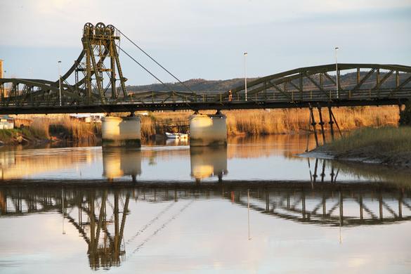
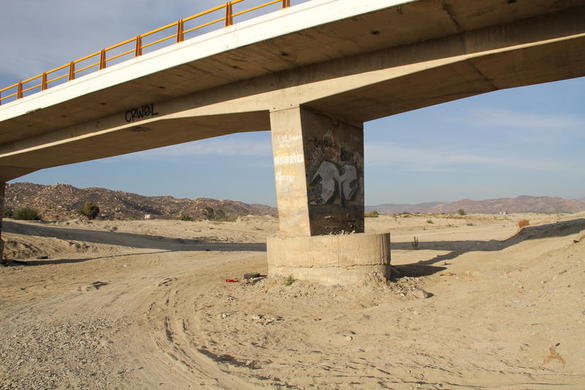
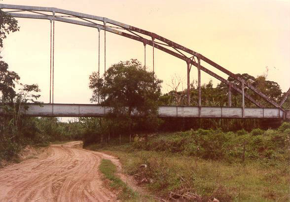
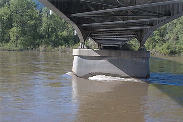
6.1 Bridge scour Bridges are road structures designed to make it possible to cross a river or stream. Bridges differ from culverts in their shape and in that they are usually much larger (Fig. 85). Generally, bridges are justified in cases of road crossings with major rivers, or when the great volume of vehicular traffic requires it. In many cases, the abutments and/or piers of the bridge are placed directly on the bed of the streams or rivers (Fig. 86), which forces the need for a stability analysis.
The stability analysis includes the study of scour of one or more piers and/or abutments of a bridge crossing. During the passage of a flood, the flow is forced to go under the bridge. The presence of one or more abutments reduces the effective cross section of the flow; therefore, the velocities increase and with this, the sediment discharge. This process eventually leads to the undermining (erosion) of the soil around the pier, which, if of sufficient magnitude, can endanger the stability of the superstructure and lead to the eventual failure of the bridge. Scour is a transient flow phenomenon which occurs during the passage of a flood. The process is dual, characterized by: (1) erosion during the rise of the flood hydrograph, and (2) deposition during the recession. In many cases, the hole produced by the erosion during the ascent is filled by the deposition during the recession. The failure occurs when the depth of the hole, called the depth of scour, is of such a magnitude that it compromises the lower level of the foundation of the structure. Therefore, the objective of the analysis is to determine the depth of scour that enables the design of the bridge foundation (in type, size and depth) with an adequate safety factor.
6.2 Types of channel degradation, scour, or erosion Scour, degradation, or erosion in the vicinity of a bridge structure may be due to one or more of the following processes:
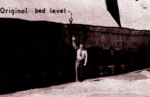
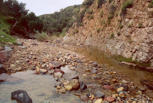
General scour is caused by a reduction in the supply of sediments in sections located upstream of the point of interest. Generally this is due to the degradation immediately downstream of a dam, caused by the phenomenon of "hungry water" (Fig. 87), or to excessive extraction of aggregates from the neighboring river beds (Fig. 88). In some cases, the reduction in the supply of sediments may be due to natural or artificial changes in the runoff coefficient of the basin located upstream.
Contraction scour usually manifests itself throughout the width of the river, during the passage of an extraordinary flood (Fig. 89).
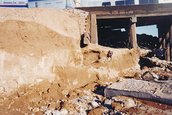
Local scour is produced by the removal of soil material around the piers, abutments, and other bridge foundation structures, caused by the acceleration of the flow in the neighborhood and the formation of vortices induced by flow obstructions. Figure 90 shows the failure of a railroad bridge near Kingman, Arizona, on August 9, 1997. The bridge failure, which led to the derailment of the train, was due to erosion and scouring of the piers and foundations of the bridge, as a result of a flood of 50-year return period (National Transportation Safety Board, 1998).
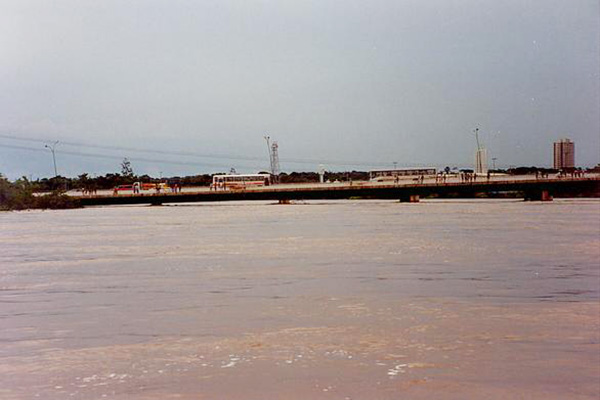
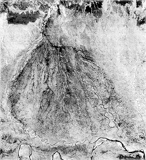
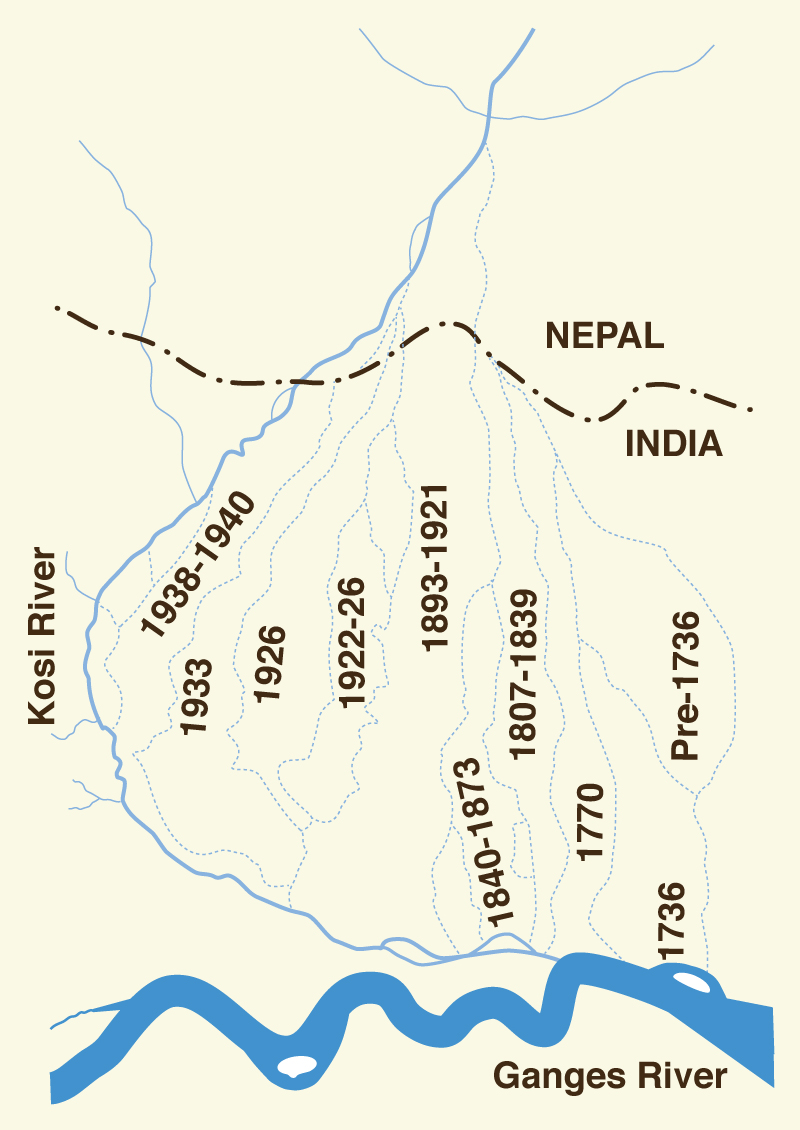
Lateral migration occurs when a river carries excessive amounts of sediment in relatively flat geomorphological situations, which forces it to fill its channel and, consequently, to look for new courses, usually during the passage of an extraordinary flood (Fig. 91). In general, any widening or lateral displacement of a fluvial channel endangers the operability of a bridge placed on it (Fig. 92). There does not seem to be a simple solution to this bridge design problem.
6.3 Contraction scour
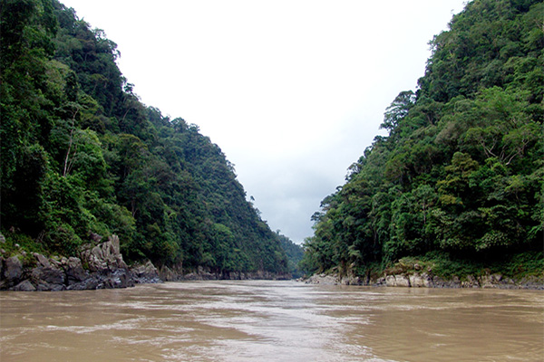
Contraction scour occurs when the flow area of a stream is reduced either: (a) by a natural contraction, or (b) by an artificial contraction due to the presence of a bridge. In most cases, contraction scour results in the deepening of the riverbed.
Figure 93 shows the Pongo de Manseriche, a natural contraction
sculpted in rock, through which the Mara��n River,
one of the two great rivers that eventually form the Amazon
River, reduces its width to 35 m as it descends the Eastern Andes Ranges, in
Amazonas, Peru. The passage through the pongo is particularly
dangerous because of the eddies that form due to the
extreme contraction of the flow, as observed in
the video
Pongo de Manseriche.
In rivers with a predominantly sandy bed, there are two types of contraction scour: (1) under clear water, and (2) under a live bed. Scouring by clear water occurs for low Froude numbers, that is, when the average velocity is less than the critical velocity necessary for the start of bed movement. In this case, the flow area in the section of the bridge, during the flood, increases until the average velocity becomes equal to the critical velocity for bed movement. Live bed scouring occurs for higher Froude numbers, for which the average velocity is greater than the critical velocity necessary for the start of bed movement. In this case, the flow area in the section of the bridge, during the flood, increases until the amount of transported material leaving the control volume is equal to that which is entering. The existing formulas for contraction scour require the determination of the type of scour. To determine if the flow immediately upstream of the bridge is producing bed movement, it is necessary to calculate the critical velocity. For this purpose, the following formula may be used:
in which: Vc = critical velocity necessary for the start of bed sediment movement, in m/sec or ft/sec; y = flow depth immediately upstream of the bridge, in m or ft; D50 = average diameter of sediment particles in the streambed, located immediately upstream of the bridge, in m or ft; and Ku = empirical constant, equal to 6.19 in the SI (metric) system, and 11.17 in the U.S. customary system of units.
To obtain the D50 of the bed material, it must be sampled in the
first 0.3 m depth.
6.3.1 Design geometry
The analysis of contraction scour depends on the particular geometrical conditions of the design.
The following cases may arise:
1.
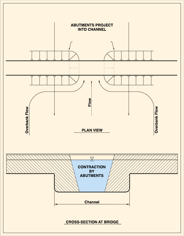
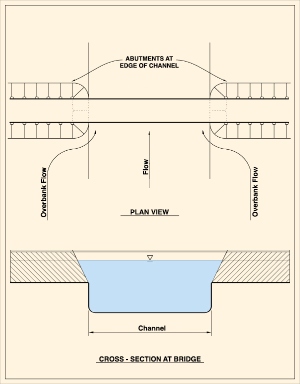
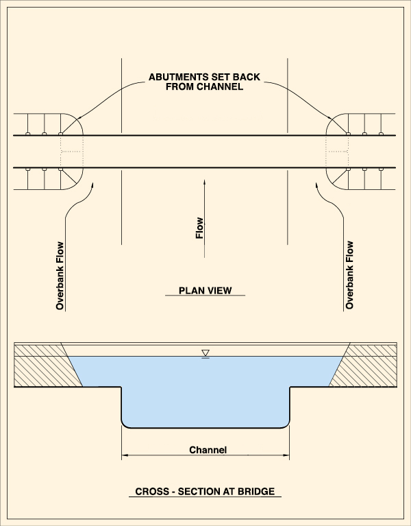
With flow in the flood plain, the distance
between the abutments is (Fig. 94):
Lesser than the width of the main channel.
Equal to the width of the main channel.
Greater than the width of the main channel..
Fig. 94 (a) Contraction scour: Case 1a.
Fig. 94 (b) Contraction scour: Case 1b.
Fig. 94 (c) Contraction scour: Case 1c.
2.
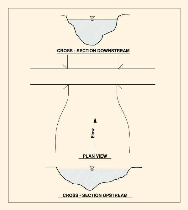
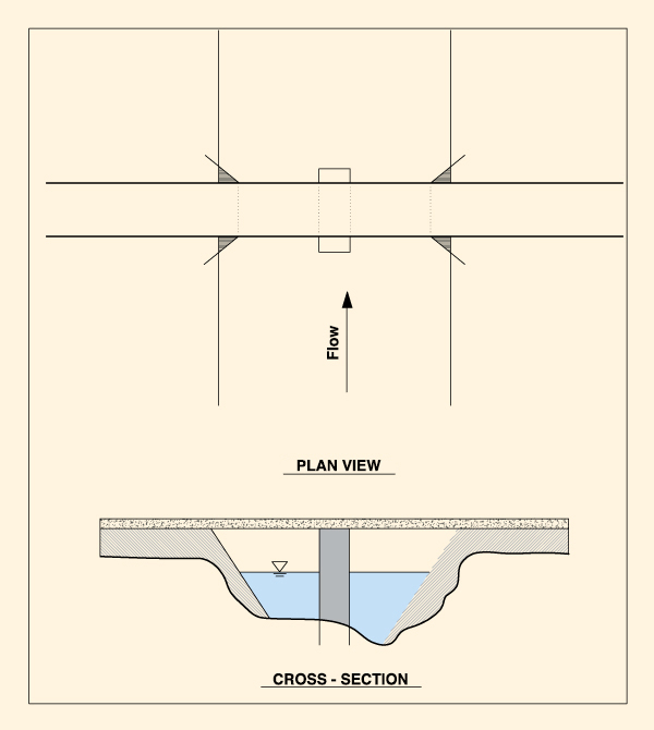
Without flow in the flood plain, the section of the stream is (Fig. 95):
Naturally narrower in the bridge and/or the section
immediately downstream.
Artificially narrower on the bridge due to obstruction caused by piers and/or abutments.
Fig. 95 (a) Contraction scour: Case 2a.
Fig. 95 (b) Contraction scour: Case 2b.
6.3.2 Contraction under live bed
The contraction scour under live
bed conditions is calculated using the modified Laursen equation (1960):
ys Q2 W1 yo
in which:
ys =
mean depth of contraction scour under live bed, in m or ft;
yo =
average depth of flow under the bridge, before scouring, in m or ft;
y1 =
mean depth immediately upstream of the bridge, in m or ft;
Q1 =
flow in the upstream section of the bridge,
which transports sediment from the bed,
comprising only the flow in the main channel, in m3/s or ft3/s;
Q2 =
flow in the contracted section, in m3/s or ft3/s;
W1 =
bottom width in the upstream section of the bridge, which transports sediment from the bed, in m or ft;
W2 =
bottom width in the contracted section, which transports sediment from the bed, in m or ft;
k1 = exponent shown in Table 23, in which:
V* = shear velocity
immediately upstream of the bridge = (gy1S1)1/2 ;
S1 = slope of the energy line in the main channel; and
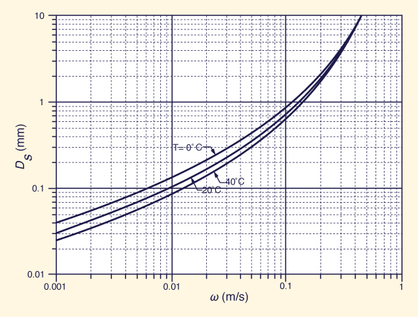
ω = fall velocity of the sediment, a function of the grain diameter
Ds (Fig. 96), that is, the mean grain diameter D50.
With reference to Eq. 201, we note the following:
6.3.3 Contraction under clear water Contraction scour under clear-water conditions is calculated using the Laursen formula (1963):
in which: ys = average depth of contraction scour under clear water, in m or ft; yo = average depth of flow under the bridge, before scour, in m or ft;
W = bottom width in the contracted section, excluding the width of the piers, in m or ft; Q = flow in the contracted section, in m3/sec o ft3/sec; Dm = diameter of the smallest sediment size in the contracted section, which is not transported, which is assumed equal to 1.25 D50, in m or ft; and Ku = empirical constant, equal to 0.025 in SI units (metric) and 0.0077 in U.S. customary units. The minimum value of D50 to use should be 0.0002 m (0.2 mm). Note that the use of a D50 value < 0.2 mm will result in an overestimation of the contraction scour under clear water.
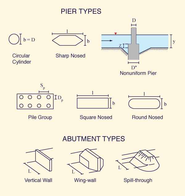
6.4 Local scour Local scour is one of the most common causes of bridge failure due to hydraulic stress. The following factors must be taken into account in the calculation of local scour in a pier or abutment:
The depth of scour increases directly with the depth and velocity of flow. Therefore, the risk of failure, usually due to an insufficient foundation depth, increases considerably during the passage of an infrequent or extraordinary flood. The depth of scour does not directly depend on the size of the bed material. However, in the case of fine materials (silt and clays), the scour velocity is usually smaller compared to that corresponding to coarse materials (sands). Established formulas for calculating local scour are the following: (1) HEC-18, (2) Jain and Fisher, (3) Froelich, and (4) Melville. These formulas are detailed below.
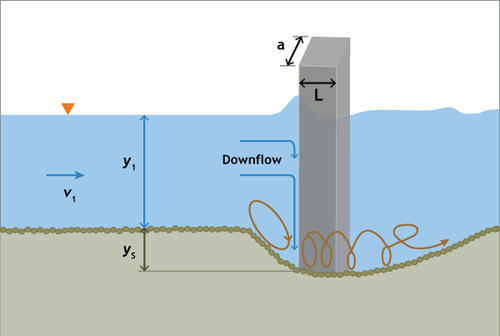
6.4.1 HEC-18 formula The HEC-18 formula calculates the maximum depth of scour in sandy fluvial beds. The formula is named after Hydraulic Engineering Circular No. 18 of the Federal Highway Administration (FHWA), of the US Department of Transportation. The HEC-18 formula is the following (Fig. 97):
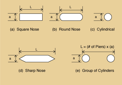
in which ys = depth of scour hole, in m; y1 = depth of flow immediately upstream of the pier, in m; v1 = mean flow velocity immediately upstream of the pier, in m/s; a = pier width, in m; F = Froude number = v1/(gy1)1/2; K1 = correction factor to take into account the shape of the cross section (Fig. 98 and Table 24); K2 = correction factor to take into account the effect of the angle θ between the alignment of the pier and the alignment of the flow (the angle of attack of the flow) (Eq. 204 or Table 25):
in which L = pier length, in m; and θ = pier attack angle; K3 = correction factor to take into account the condition of the fluvial bed (Table 26).
6.4.2 Jain and Fisher formula The Jain and Fisher formula is applicable to the calculation of local scour. The formula distinguishes between two types of scour:
The formulas are the following: a. Scour under clear water, for the case (F - Fc ) ≤ 0.2:
b. Scour under live bed, for the case (F - Fc ) > 0.2:
in which: ys = depth of scour; a = pier width; v = mean velocity of the flow immediately upstream; y = depth of flow immediately upstream; Vc = critical velocity, at which bed sediment movement starts; F = Froude number = v/(gy)0.5; and Fc = critical Froude number = Vc /(gy)0.5. The critical velocity may be estimated using the following.
in which: Vc = critical velocity necessary for the start of bed sediment movement, in m/sec or ft/sec; y = depth of flow immediately upstream of the bridge, in m or ft; D50 = mean diameter of the bed sediment particles located immediately upstream of the bridge, in m or ft; Ku = empirical constant, equal to 6.19 in the SI system (metric), and 11.17 in the U.S. customary system of units; To obtain the D50 of the bed material, it must be sampled in the first 0.3 m depth. Eq. 206a is applicable to granular materials, being restricted to values of D50 ≥ 0.0002 m (0.2 mm). For smaller sizes, cohesion has the effect of increasing the critical velocity.
6.4.3 Froehlich's formula
Froehlich's formula is frequently used for the calculation of local scour in a bridge pier
in which: ys = scour depth (L units); b = pier width (L units); D50 = mean particle diameter (L units); be = projection of the pier width b in a plane normal to the angle of attack θ (L units);
φ = dimensionless coefficient
which accounts for the form
of the cross section v1 = mean velocity immediately upstream of the pier (L /T units); y1 = flow depth immediately upstream of the pier (L units); Fr1 = Froude number immediately upstream of the pier: Fr1 = v1 /(gy1)0.5; Equation 207 is dimensionless when used with consistent units (m or ft).
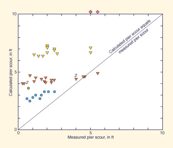
Figure 100 shows an evaluation of Eq. 207. Note that the calculated values are almost always greater than the measured values. Also, note that Froehlich's formula is one of those included in HEC-RAS.
6.4.4 Melville's formula Melville's formula calculates the maximum depth of local scour on a bridge pier or abutment. The formula is based on a product of six empirical variables K, each of which evaluates a contributing factor to local scour. The formula is:
in which: ds = maximum depth of local scour, in units of length (m or ft); KyW = depth factor: (a) Kyb for piers, o (b) KyL for abutments, in units of length (m or ft); KI = factor of flow intensity, including effects of sediment gradation and flow velocity, dimensionless; Kd = factor of sediment size; dimensionless; Ks = factor of shape of the pier or abutment; dimensionless; Kθ = factor of alignment of the pier or abutment; dimensionless; and KG = factor of geometry of the canal; dimensionless. Equation 208 evaluates the local scour of piers or abutments in cases where contraction scour is negligible. Depth factor for piers or abutments The depth factor KyW (Kyb for piers or KyL abutments) is given by one of the following equations:
in which: y = flow depth immediately upstream of the pier or abutment; b = pier width; y L = abutment length, including the bridge approximation, projected in a direction perpendicular to the flow. Flow intensity factor Regarding the flow intensity factor, it is necessary to distinguish between two types of local scour: (1) under clear water, and (2) under live bed, as in the case of the Jain and Fisher formula (Section 6.4.2). Scouring under clear water occurs before the start of the movement of the bed, and scour under live bed after the start of movement.
Scouring under clear water typically occurs in the floodplain.
Scouring under live bed occurs when there is sediment transport in the
vicinity of the hole. If the sediment is uniform, that is, with a gradation coefficient
The flow intensity factor KI is given by one of the following equations:
in which: V = mean flow velocity immediately upstream; Vc = mean flow velocity immediately upstream, at the onset of bed movement; Va = mean flow velocity immediately upstream, at the start of live bed movement (for uniform sediments, Va = Vc; for nonuniform sediments, Va > Vc); Va = 0.8 Vca; and Vca = mean flow velocity beyond which armoring of a nonuniform sediment bed is impossible The velocities Vc and Vca are calculated with the following formulas:
in which: d50 = mean particle diameter (mm); d50a = dmax / 1.8; and dmax = máximum particle diameter (mm). For quartz sediments at the temperature of T = 20°C, the shear velocities u*c y u*ca are estimated as follows:
Factor of sediment size The factor of sediment size Kd is given by one of the following equations:
in which W = b for piers, and W = L for abutments. Factor of shape of the pier or abutment The shape factor Ks is shown in Table 27, with reference to Fig. 101.
For long abutments, the shape factor is not too important. Therefore, the factor Ks shown in Table 26 should be replaced by the following modified factor K*s:
Factor of alignment of the pier or abutment
The alignment factor Kθ
is shown in Table 28. Note that for the case of piers,
these values are the same as the correction factors K1
shown in
The factor Kθ for abutments applies only for the case of long abutments. Therefore, this value is to be replaced by the following modified factor K*θ :
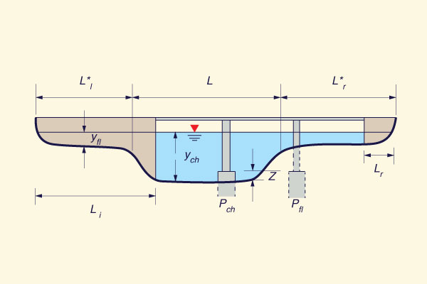
Factor of geometry of the canal In the case of a pier, the geometry of the canal does not affect the amount of scour. Therefore, the factor of geometry for a pier is KG = 1. In the case of an abutment, the factor of geometry KG is given by the following formula: Left abutment
in which (Fig. 102): Li = length of left abutment; L*i = width of the flood plain on the left abutment; y = flow depth in the main channel; y*i = flow depth in the flood plain on the left abutment; n = Manning coefficient in the main channel; and n*i = Manning coefficient in the flood plain of the left abutment. Right abutment
in which (Fig. 102): Li = length of right abutment; L*i = width of the flood plain on the right abutment; y = flow depth in the main channel; y*i = flow depth in the flood plain on the right abutment; n = Manning coefficient in the main channel; and n*i = Manning coefficient in the flood plain of the right abutment.
6.5 Unconventional stream crossings
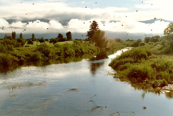
In nature, rivers are classified into: (1) perennial, (2)
intermittent, and (3) ephemeral. Perennial rivers always
have water, which originates in the baseflow [Fig. 103 (a)].
Intermittent rivers have water only a few months a year,
with low water flows sustained by seasonal groundwater
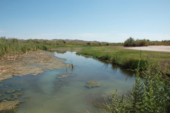
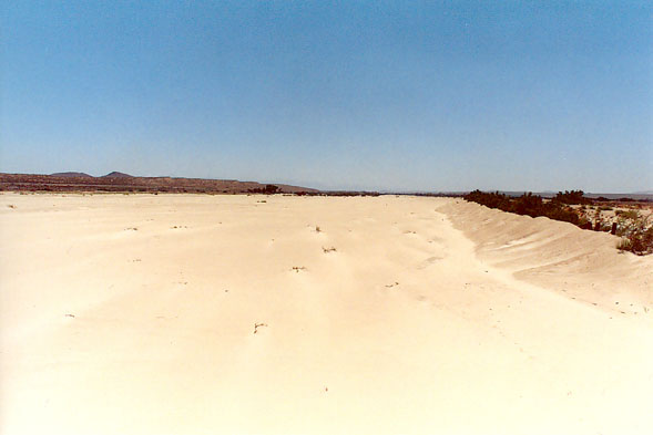
flows [Figs. 103 (b) and (c)]. Ephemeral rivers have
water only during and immediately following a precipitation
event [Fig. 103 (d)]. The position of the water table,
above, at the level, or below the streambed,
determines if it is perennial, intermittent, or ephemeral, respectively.
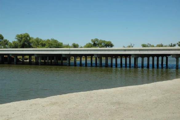
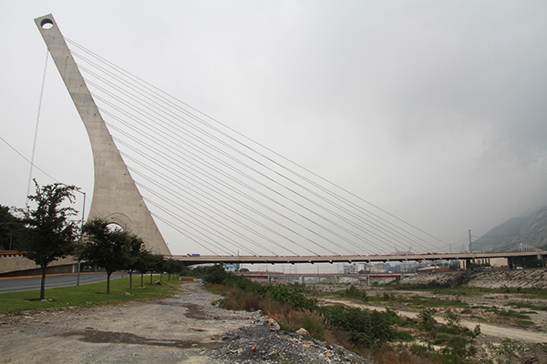
The depth to the water table varies across the climatic spectrum, from arid regions to humid regions. In humid areas, the water table is close to the surface, while in arid areas it is found at much greater depths. In general, the drier the climate, the greater the depth to the water table. Therefore, ephemeral rivers are quite common in arid regions. The peak of erosion and sediment transport occurs around an average annual precipitation of 375 mm (15 inches), which corresponds to an arid region (200-400 mm) (Ponce et al., 2000). Therefore, rivers located in arid regions usually transport large amounts of sediment. From a geomorphological perspective, when a river carries a large amount of sediments, the width-depth ratio is large, typically between 50 and 100. Therefore, river crossings in arid regions represent a considerable challenge for design. The problem is how to make possible the crossing of an ephemeral river in an effective and economic way. River bridges can be of various types; in principle they must cover the entire width of the river (Fig. 104). When the bridges do not cover the entire width of the river, this leads to problems during the floods. Generally, during a flood the river reclaims its actual width, endangering the foundation and, consequently, the stability of the structure. Excessive speeds in the vicinity of piers or abutments can cause local erosion and lead to the eventual failure of the bridge.
The bridges are built when the volume of traffic and/or the importance of the road network justify the cost. Most bridges are permanent structures, vulnerable to extreme floods. Rivers, particularly those located in arid regions, can overflow their channels, or even change course, making the crossing structure inoperable (Fig. 92).
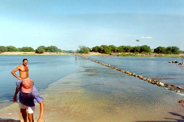
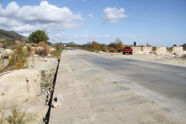
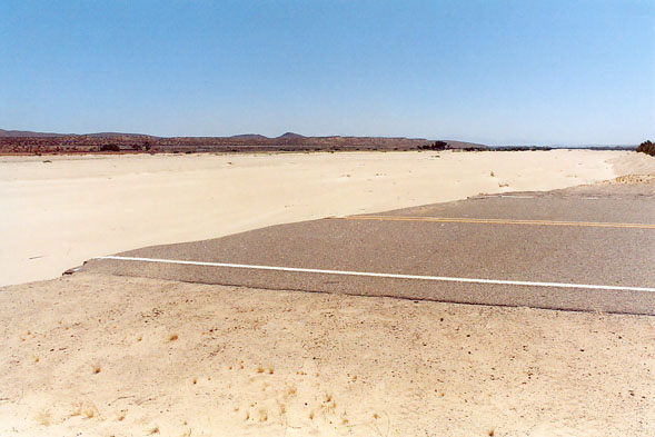
6.5.1 The ford crossing A ford is a temporary or permanent structure to cross a river or stream, without the full benefit of a bridge. The ford is a design alternative in cases of light traffic or limited resources. The constructed fords are designed to cross the river on a concrete slab for cases where the flow is small or non-existent (Fig. 105). In arid regions, fords are common in places where water flows only a few days out of the year (Fig. 106). The ford is an economical way to solve the problem of crossing a river.
The disadvantage of a ford is that it may be out of service a few days out of the year, but when this is compared to the cost of a bridge, the decision may be justified. Fords are generally used in rural areas, where traffic and/or economic resources are limited.
A singular case of the crossing of an important river by
means of a built ford is that of
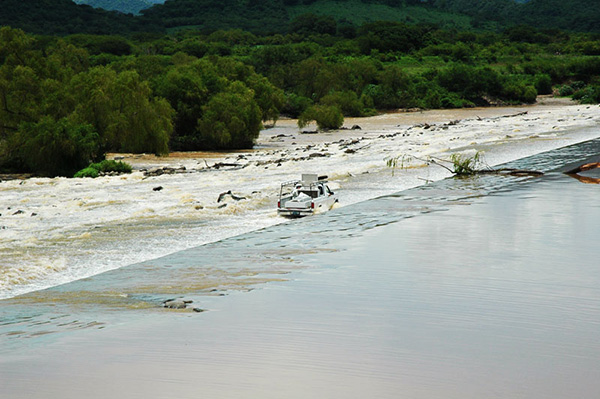
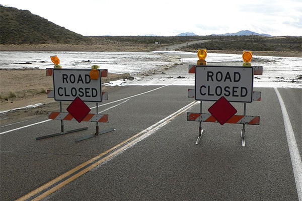
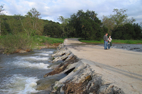
During extraordinary floods, fords are also subject, like bridges, to hydraulic erosion, possible failure and consequent inoperability. Figure 109 shows a ford on Indian Trail Road, on the Mojave River, near Helendale, California: (a) during the failure, in March 2005, and (b) some time after the failure.
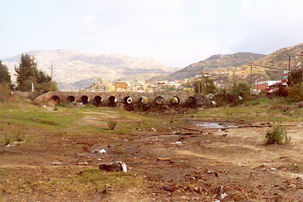
6.5.2 The Arizona crossing The Arizona crossing is a type of ford used in the southwest of the United States for the crossing of ephemeral river channels. The ford consists of a predetermined group of circular culverts, usually of corrugated aluminum, aligned to form an embankment, enabling the passage of vehicles on top of it (Fig. 110). The length of the embankment usually comprises the main channel of the stream or river. This type of crossing is designed for a limited overflow in the case of an infrequent or extraordinary flood. There is the possibility of partial or total failure of the embankment as a result of excessive erosion during a major flood.
The culvert bridge (Fig. 111) is similar to the Arizona crossing. The difference is that the culvert bridge is not designed for an eventual spillover. During an extraordinary flood, the overflow may endanger the integrity of the structure.
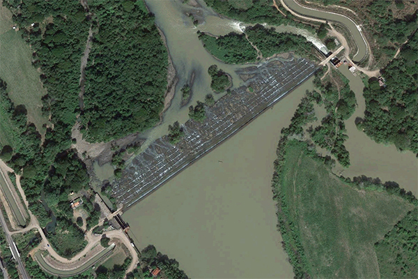
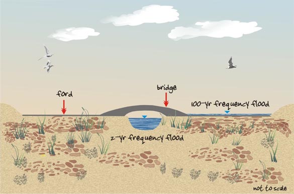
6.5.3 The ford-bridge A ford-bridge is a combination of ford and bridge, with a maximum of advantages and a minimum of disadvantages. The ford-bridge is designed to work as a bridge during periods of low flow and as a ford during high flows. In an ephemeral river, a ford-bridge resembles a ford for the most part, but contains a relatively small bridge, designed to pass the mean annual flood (Fig. 112).
The ford-bridge can span at comparatively small cost the total width of the river. There is no need to shorten the width of the structure and there are no bridge piers that can fail during an extraordinary flood. Essentially, the ford-bridge works as a ford during extraordinary floods; at all other times, the ford-bridge serves as a bridge. For ephemeral rivers in arid regions, the ford-bridge provides a suitable combination of functionality and economy. All river crossings are designed to sustain a specific hydrologic load. This is usually the 100-yr flood, and in some cases, even greater. In a typical bridge design, peak flow is expressed in terms of depths and velocities and these data are used to calculate local scour on piers and abutments. In contrast, a ford has no piers; the only design requirement is the proper anchoring of the slab to minimize the possibility of lifting [Note the lack of an anchored slab in Fig. 109 (a)]. As in the case of a bridge, the possibility of failure always exists during extreme floods. The components of a ford-bridge must be designed as fords and bridges, respectively. The design of the ford component is of the conventional type; however, the bridge component is much smaller than a typical bridge. The design of the bridge may be based on the average annual flood, that is, the 2-yr flood, which, from a geomorphological perspective, is formative of the main channel. This contrasts with the 100-yr flood used in the design of conventional bridges. During extreme events, the ford distributes the hydraulic load across the entire channel width. Therefore, the ford-bridge is in an optimal position to withstand the loads and stresses typical of extraordinary floods.
The ford-bridge is a practical alternative to the conventional bridge or ford. The concept is applicable in ephemeral
rivers featuring a large width-to-depth ratio, particularly in rural areas, or where traffic is light and resources are
limited. The design of the ford-bridge optimizes the hydrologic loads, using the bridge for the 2-yr flood
and the ford for the
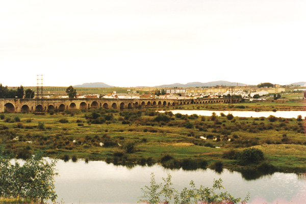
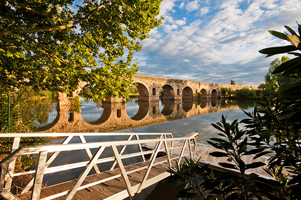
6.6 Longevity of a bridge Based on what is presented in Sections 6.3 to 6.5, it can be concluded that the longevity of a bridge depends on whether its as-built length respects the hydraulic integrity of the river it crosses. For example, the Roman bridge over the Guadiana river, in Merida, Spain, dating back to the 1st century B.C., is still in operation (although only in the pedestrian mode), having been partially restored several times (Fig. 113). With a height of 12 m and a length of 792 m in 60 arches, the bridge occupies a large part of the floodplain of the large and regionally important Guadiana river.
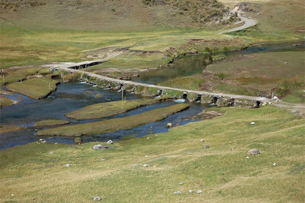
Another example of bridge longevity is the ancient Inca bridge, located near the headwaters of the Lauricocha River, in Huanuco, Peru, for which an age of more than 500 years has been reported. Figure 114 clearly shows that this bridge, 60 m long and with a total of 24 bays, is approximately six (6) times longer than the dry-season width of the river.
|
||||||||||||||||||||||||||||||||||||||||||||||||||||||||||||||||||||||||||||||||||||||||||||||||||||||||||||||||||||||||||||||||||||||||||||||||||||||||||||||||||||||||||||||||||||||||||||||||||||||||||||||||||||||||||||||||||||||||||||||||||||||||||||||||||||||||||||||||||||||||||||||||||||||||||||||||||||||||||||||||||||||||||||||||||||||||||||||||||||||||||||||||||||||

| ruler |