CIVE 530 - OPEN-CHANNEL HYDRAULICS LECTURE 13: HEC-RAS, Chapter 2, Theoretical basis for one-dimensional flow calculations

THEORETICAL BASIS FOR ONE-DIMENSIONAL FLOW CALCULATIONS

This chapter describes the methodologies used in performing the one-dimensional flow calculations within HEC-RAS. The basic equations are presented along with discussions of the various terms. Solution schemes for the various equations are described. Discussions are provided as to how the equations should be applied, as well as applicable limitations. Contents General Steady Flow Water Surface Profiles Unsteady Flow Routing (not included here)

STEADY-FLOW WATER-SURFACE PROFILES

HEC-RAS is currently capable of performing one-dimensional water surface profile calculations for steady gradually varied flow in natural or constructed channels. Subcritical, supercritical, and mixed flow regime water surface profiles can be calculated. Topics discussed in this section include: equations for basic profile calculations cross section subdivision for conveyance calculations composite Manning's n for the main channel velocity weighting coefficient alpha friction loss evaluation contraction and expansion losses computational procedure critical depth determination applications of the momentum equation limitations of the steady flow model.

EQUATIONS FOR BASIC PROFILE CALCULATION

Water surface profiles are computed from one cross section to the next by solving the energy equation with an iterative procedure called the standard step method. The energy equation is written as follows: Y2 + Z2 + α2[V22 /(2g)] = Y1 + Z1 + α1[V12 /(2g)] + he in which: Y1, Y2 = flow depth at cross sections Z1, Z2 = elevation of the main channel inverts V1, V2 = average velocities (total discharge / total flow area) &alpha1, α2 = velocity weighting coefficients g = gravitational acceleration he = energy head loss A diagram showing the terms of the energy equation is shown in Figure 2-1. Figure 2.1   Representation of terms in the energy equation. The energy head loss (he) between two cross sections is comprised of friction losses and contraction/expansion losses. The equation for the energy head loss is as follows: he = L Sfbar + C | α2[V22 /(2g)] - α1[V12 /(2g)] | in which: L = discharge-weighted reach length S fbar = representative (average) friction slope between two sections C = expansion (or contraction) loss coefficient The distance weighted reach length, L, is calculated as follows: L = [ Llob Qlob + Lch Qch + Lrob Qrob ] / [ Qlob + Qch + Qrob ] in which: Llob, Lch, Lrob = cross section reach lengths specified for flow in the left overbank, main channel, and right overbank, respectively Qlob, Qch, Qrob = flows between sections for the left overbank, main channel, and right overbank, respectively

CROSS SECTION SUBDIVISION FOR CONVEYANCE CALCULATIONS

The determination of total conveyance and the velocity coefficient for a cross section requires that flow be subdivided into units for which the velocity is uniformly distributed. The approach used in HEC-RAS is to subdivide flow in the overbank areas using the input cross section n-value break points (locations where n-values change) as the basis for subdivision (Figure 2-2). Conveyance is calculated within each subdivision from the following form of Manning's equation (based on U.S. Customary units): Q = K S f1/2 K = (1.486/n) A R2/3 in which: K = conveyance for subdivision n = Manning's roughness coefficient for subdivision A = flow area for subdivision R = hydraulic radius for subdivision (area / wetted perimeter) The program sums up all the incremental conveyances in the overbanks to obtain a conveyance for the left overbank and the right overbank. The main channel conveyance is normally computed as a single conveyance element. The total conveyance for the cross section is obtained by summing the three subdivision conveyances (left, channel, and right). Figure 2.2   HEC-RAS default conveyance subdivision method. An alternative method available in HEC-RAS is to calculate conveyance between every coordinate point in the overbanks (Figure 2.3). The conveyance is then summed to get the total left overbank and right overbank values. This method is used in the Corps HEC-2 program. The method has been retained as an option within HEC-RAS in order to reproduce studies that were originally developed with HEC-2. Figure 2.3   Alternative conveyance subdivision method (HEC-2 style). DIFFERENCES BETWEEN THE TWO METHODS OF COMPUTING CONVEYANCE The two methods for computing conveyance will produce different answers whenever portions on the overbank have ground sections with significant vertical slopes. In general, the HEC-RAS default approach will provide a lower total conveyance for the same water surface elevation. In order to test the significance of the two ways of computing conveyance, comparisons were performed using 97 data sets from the HEC profile accuracy study (HEC, 1986). Water surface profiles were computed for the 1% chance event using the two methods for computing conveyance in HEC-RAS. The results of the study showed that the HEC-RAS default approach will generally produce a higher computed water surface elevation. Out of the 2048 cross section locations, 47.5% had computed water surface elevations within 0.10 ft. (30.48 mm), 71% within 0.20 ft. (60.96 mm), 94.4% within 0.4 ft. (121.92 mm), 99.4% within 1.0 ft. (304.8 mm), and one cross section had a difference of 2.75 ft. (0.84 m). Because the differences tend to be in the same direction, some effects can be attributed to propagation of downstream differences. The results from the conveyance comparisons do not show which method is more accurate; they only show differences. In general, it is felt that the HECRAS default method is more commensurate with the Manning equation and the concept of separate flow elements. Further research, with observed water surface profiles, will be needed to make any conclusions about the accuracy of the two methods.

COMPOSITE MANNING'S n FOR THE MAIN CHANNEL

Flow in the main channel is not subdivided, except when the roughness coefficient is changed within the channel area. HEC-RAS tests the applicability of subdivision of roughness within the main channel portion of a cross section, and if it is not applicable, the program will compute a single composite n value for the entire main channel. The program determines if the main channel portion of the cross section can be subdivided or if a composite main channel n value will be utilized based on the following criterion: if a main channel side slope is steeper than 5H:1V and the main channel has more than one n-value, a composite roughness nc will be computed [Equation 6-17, Chow, 1959]. The channel side slope used by HEC-RAS is defined as the horizontal distance between adjacent n-value stations within the main channel over the difference in elevation of these two stations (see SL and SR of Figure 2.4). Figure 2.4   Definition of bank slope for composite nc calculation. For the determination of nc, the main channel is divided into N parts, each with a known wetted perimeter Pi and roughness coefficient ni. n = [ ∑i=1N (Pi ni3/2 ) / P ]2/3 in which: nc = composite or equivalent coefficient of roughness P = wetted perimeter of entire main channel Pi = wetted perimeter of subdivision I ni = coefficient of roughness for subdivision I The computed composite nc should be checked for reasonableness. The computed value is the composite main channel n value in the output and summary tables.

EVALUATION OF THE MEAN KINETIC ENERGY HEAD

Because the HEC-RAS software is a one-dimensional water surface profiles program, only a single water surface and therefore a single mean energy are computed at each cross section. For a given water surface elevation, the mean energy is obtained by computing a flow weighted energy from the three subsections of a cross section (left overbank, main channel, and right overbank). Figure 2.5 below shows how the mean energy would be obtained for a cross section with a main channel and a right overbank (no left overbank area). Figure 2.5   Example of how mean energy is obtained. To compute the mean kinetic energy it is necessary to obtain the velocity head weighting coefficient α. α is calculated as follows: α = [ ∑iN QiVi2 ] / (Qt Vt2) The velocity coefficient α can also be written in terms of conveyance and flow area as in the following equation: α = [ ∑iN Ki3/Ai2 ] / (Kt3/At2 ) in which: K = conveyance, A = flow area, and i = lob, ch, and rob (left overbank, channel, and right overbank, respectively.

FRICTION LOSS EVALUATION

Friction loss is evaluated in HEC-RAS as the product of Sf and L. Sf is the representative friction slope for a reach. L is the discharge-weighted reach length. The friction slope (slope of the energy gradeline) at each cross section is computed from Manning's equation as follows: Sf = (Q/K) 2 Alternative expressions for the representative-reach friction slope (Sf) in HEC-RAS are as follows: Average conveyance equation Sf bar = [ (Q1 + Q2) /(K1 + K2) ]2 Average friction slope equation Sf bar = ( Sf1 + Sf2 ) / 2 Geometric mean friction slope equation Sf bar = ( Sf1 × Sf2 ) 1/2 Harmonic mean friction slope equation Sf bar = 2 ( Sf1 × Sf2 ) / ( Sf1 + Sf2 ) The average conveyance equation is the default method used by the program; that is, it is used automatically unless a different equation is requested by input. The program also contains an option to select equations, depending on flow regime and profile type (e.g., S1, M1, etc.).

CONTRACTION AND EXPANSION LOSS EVALUATION

Contraction and expansion losses in HEC-RAS are evaluated by the following equation: hce = C | (&alpha1V12)/(2g) - (&alpha1V12)/(2g) | in which: C = the contraction or expansion coefficient. The program assumes that a contraction is occurring whenever the velocity head downstream is greater than the velocity head upstream. Likewise, when the velocity head upstream is greater than the velocity head downstream, the program assumes that a flow expansion is occurring.

COMPUTATION PROCEDURE

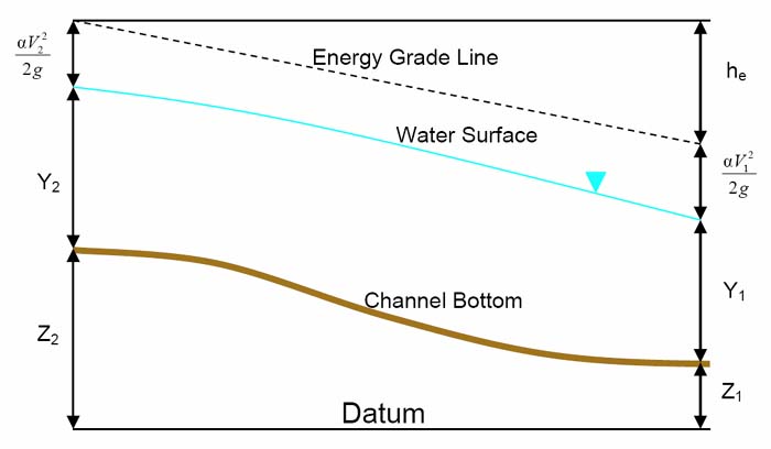
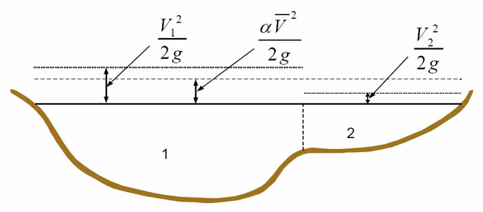
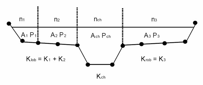
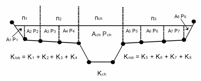
The unknown water surface elevation at a cross section is determined by an iterative solution of the gradually varied flow equation (Equation 2-1) and the energy head loss equation (Equation 2-2). The computational procedure is as follows: Assume a water surface elevation WS2 at the upstream cross section (or downstream cross section if a supercritical profile is being calculated). Based on the assumed water surface elevation, determine the corresponding total conveyance and velocity head. With values from step 2, compute Sf and solve Equation 2-2 for he. With values from steps 2 and 3, solve Equation 2-1 for WS2. Compare the computed value of WS2 with the value assumed in step 1; repeat steps 1 through 5 until the values agree to within .01 feet (.003 m), or the user-defined tolerance. The criterion used to assume water surface elevations in the iterative procedure varies from trial to trial. The first trial water surface is based on projecting the previous cross section's water depth onto the current cross section. The second trial water surface elevation is set to the assumed water surface elevation plus 70% of the error from the first trial (computed W.S. - assumed W.S.). In other words, W.S. new = W.S. assumed + 0.70 * (W.S. computed - W.S. assumed). The third and subsequent trials are generally based on a "Secant" method of projecting the rate of change of the difference between computed and assumed elevations for the previous two trials. The change from one trial to the next is constrained to a maximum of 50% of the assumed depth from the previous trial. On occasion the secant method can fail if the value of error difference becomes too small. If the error difference is less than 0.01, then the secant method is not used. When this occurs, the program computes a new guess by taking the average of the assumed and computed water surfaces from the previous iteration. 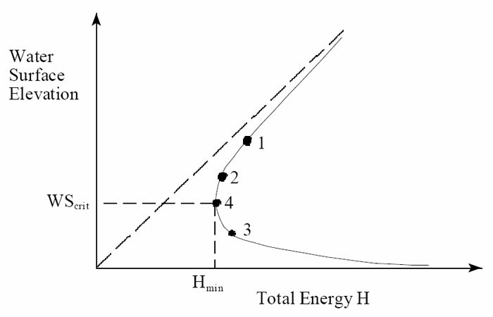The program is constrained by a maximum number of iterations (the default is 20) for balancing the water surface. While the program is iterating, it keeps track of the water surface that produces the minimum amount of error between the assumed and computed values. This water surface is called the minimum error water surface. If the maximum number of iterations is reached before a balanced water surface is achieved, the program will then calculate critical depth (if this has not already been done). The program then checks to see if the error associated with the minimum error water surface is within a predefined tolerance (the default is 0.3 ft or 0.1 m). If the minimum error water surface has an associated error less than the predefined tolerance, and this water surface is on the correct side of critical depth, then the program will use this water surface as the final answer and set a warning message that it has done so. If the minimum error water surface has an associated error that is greater than the predefined tolerance, or it is on the wrong side of critical depth, the program will use critical depth as the final answer for the cross section and set a warning message that it has done so. The rationale for using the minimum error water surface is that it is probably a better answer than critical depth, as long as the above criteria are met. Both the minimum error water surface and critical depth are only used in this situation to allow the program to continue the solution of the water surface profile. Neither of these two answers are considered to be valid solutions, and therefore warning messages are issued when either is used. In general, when the program cannot balance the energy equation at a cross section, it is usually caused by an inadequate number of cross sections (cross sections spaced too far apart) or bad cross section data. Occasionally, this can occur because the program is attempting to calculate a subcritical water surface when the flow regime is actually supercritical. When a balanced water surface elevation has been obtained for a cross section, checks are made to ascertain that the elevation is on the right side of the critical water surface elevation (e.g., above the critical elevation if a subcritical profile has been requested by the user). If the balanced elevation is on the wrong side of the critical water surface elevation, critical depth is assumed for the cross section and a warning message to that effect is displayed by the program. The program user should be aware of critical depth assumptions and determine the reasons for their occurrence, because in many cases they result from reach lengths being too long or from misrepresentation of the effective flow areas of cross sections. For a subcritical profile, a preliminary check for proper flow regime involves checking the Froude number. The program calculates the Froude number of the balanced water surface for both the main channel only and the entire cross section. If either of these two Froude numbers are greater than 0.94, then the program will check the flow regime by calculating a more accurate estimate of critical depth using the minimum specific energy method (this method is described in the next section). A Froude number of 0.94 is used instead of 1.0, because the calculation of Froude number in irregular channels is not accurate. Therefore, using a value of 0.94 is conservative, in that the program will calculate critical depth more often than it may need to. For a supercritical profile, critical depth is automatically calculated for every cross section, which enables a direct comparison between balanced and critical elevations.

CRITICAL DEPTH DETERMINATION

Critical depth for a cross section will be determined if any of the following conditions are satisfied: The supercritical flow regime has been specified. The calculation of critical depth has been requested by the user. This is an external boundary cross section and critical depth must be determined to ensure the user entered boundary condition is in the correct flow regime. The Froude number check for a subcritical profile indicates that critical depth needs to be determined to verify the flow regime associated with the balanced elevation. The program could not balance the energy equation within the specified tolerance before reaching the maximum number of iterations. The total energy head for a cross section is defined by: H = WS + &alpha V2/(2g) in which: H = total energy head. WS = water surface elevation. &alpha V2/(2g) = velocity head. The critical water surface elevation is the elevation for which the total energy head is a minimum. The critical elevation is determined with an iterative procedure whereby values of WS are assumed and corresponding values of H are determined with the above equation until a minimum value for H is reached. Figure 2.6   Energy vs water-surface elevation diagram. The HEC-RAS program has two methods for calculating critical depth: a parabolic method and a secant method. The parabolic method is computationally faster, but it is only able to locate a single minimum energy. For most cross sections there will only be one minimum on the total energy curve, therefore the parabolic method has been set as the default method (the default method can be changed from the user interface). If the parabolic method is tried and it does not converge, then the program will automatically try the secant method. PARABOLIC VS SECANT METHOD In certain situations it is possible to have more than one minimum on the total energy curve. Multiple minimums are often associated with cross sections that have breaks in the total energy curve. These breaks can occur due to very wide and flat overbanks, as well as cross sections with levees and ineffective flow areas. When the parabolic method is used on a cross section that has multiple minimums on the total energy curve, the method will converge on the first minimum that it locates. This approach can lead to incorrect estimates of critical depth. If the user thinks that the program has incorrectly located critical depth, then the secant method should be selected and the model should be re-run. The "parabolic" method involves determining values of H for three values of WS that are spaced at equal ΔWS intervals. The WS corresponding to the minimum value for H, defined by a parabola passing through the three points on the H versus WS plane, is used as the basis for the next assumption of a value for WS. It is presumed that critical depth has been obtained when there is less than a 0.01 ft. (0.003 m) change in water depth from one iteration to the next, and provided the energy head has not either decreased or increased by more than .01 feet (0.003 m). PROCEDURE FOR THE SECANT METHOD The secant method first creates a table of water surface versus energy by slicing the cross section into 30 intervals. If the maximum height of the cross section (highest point to lowest point) is less than 1.5 times the maximum height of the main channel (from the highest main channel bank station to the invert), then the program slices the entire cross section into 30 equal intervals. If this is not the case, the program uses 25 equal intervals from the invert to the highest main channel bank station, and then 5 equal intervals from the main channel to the top of the cross section. The program then searches this table for the location of local minimums. When a point in the table is encountered such that the energy for the water surface immediately above and immediately below are greater than the energy for the given water surface, then the general location of a local minimum has been found. The program will then search for the local minimum by using the secant slope projection method. The program will iterate for the local minimum either thirty times or until the critical depth has been bounded by the critical error tolerance. After the local minimum has been determined more precisely, the program will continue searching the table to see if there are any other local minimums. The program can locate up to three local minimums in the energy curve. If more than one local minimum is found, the program sets critical depth equal to the one with the minimum energy. If this local minimum is due to a break in the energy curve caused by overtopping a levee or an ineffective flow area, then the program will select the next lowest minimum on the energy curve. If all of the local minimums are occurring at breaks in the energy curve (caused by levees and ineffective flow areas), then the program will set critical depth to the one with the lowest energy. If no local minimums are found, then the program will use the water surface elevation with the least energy. If the critical depth that is found is at the top of the cross section, then this is probably not a real critical depth. Therefore, the program will double the height of the cross section and try again. Doubling the height of the cross section is accomplished by extending vertical walls at the first and last points of the section. The height of the cross section can be doubled five times before the program will quit searching.

APPLICATIONS OF THE MOMENTUM EQUATION

Whenever the water surface passes through critical depth, the energy equation is not considered to be applicable. The energy equation is only applicable to gradually varied flow situations, and the transition from subcritical to supercritical or supercritical to subcritical is a rapidly varying flow situation. There are several instances when the transition from subcritical to supercritical and supercritical to subcritical flow can occur. These include significant changes in channel slope, bridge constrictions, drop structures and weirs, and stream junctions. In some of these instances empirical equations can be used (such as at drop structures and weirs), while at others it is necessary to apply the momentum equation in order to obtain an answer. Within HEC-RAS, the momentum equation can be applied for the following specific problems: the occurrence of a hydraulic jump; low flow hydraulics at bridges; and stream junctions. In order to understand how the momentum equation is being used to solve each of the three problems, a derivation of the momentum equation is shown here. The application of the momentum equation to hydraulic jumps and stream junctions is discussed in detail in Chapter 4. Detailed discussions on applying the momentum equation to bridges is discussed in Chapter 5.

051128