• The Earth's atmosphere contains water vapor.

• The amount of vapor is expressed as a depth of precipitable water.

• The amount of water vapor contained in the air is a function of the temperature.

• Lowering of the temperature reduces the amount of water vapor that the air can contain. The rest is precipitated.

• Cooling of air masses can be due to:
  
  
  • Horizontal convergence lifting: moist air masses move to low-pressure area, collide, vapor raises, and cooling results.

  • Frontal lifting: warm moist air moves into colder air, which acts as a wedge; warm air rises, and cooling results.

  • Orographic lifting: moist air flows toward an orographic barrier and is forced to rise, resulting in its cooling.

  • Longwave-radiation lifting: in heavily vegetated regions, with low albedo, excess longwave radiation warms moist air and results in its lifting.

• Condensed water vapor must attain precipitation size in order to precipitate.

• Air particles such as aerosols trigger coalescence of condensed water vapor into rain drops.

• Factors affecting precipitation  (Link 4203).

Quantitative description of rainfall

• Rain consists of liquid-water drops, mostly larger than 0.5 mm in diameter.

• Rainfall intensities can be light (less than 3 mm/hr) to heavy (more than 10 mm/hr).

• Snow is ice crystals.

• Hail is solid icestones, from 5 to 125 mm in diameter.

• Rainfall durations of 1, 2, 3, 6, 12, and 24 hr are common.

• Rainfall depths can vary widely, depending on climate and season.

• Larger depths occur more infrequently.

• For example: a 60 mm rainfall lasting 6 hr may occur once every 10 yr (Intensity-Duration-Frequency).

• Return period is the reciprocal of the frequency: once in 50 yr (1/50) means a 50 yr return period.

• For long return periods, data is lacking to support statistical analysis (more than 100 years).

• Deterministic concept of PMP (Probable Maximum Precipitation) takes over in the U.S.

• PMP leads to PMF (Probable Maximum Flood).

• SPF (Standard Project Flood) is a fraction of the PMF (Corps of Engineers practice).

• Q&A on the return period to be used for design. (Link 4221).

Temporal rainfall distribution

• Variation of rainfall depth within the event duration is depicted by the temporal rainfall distribution.

• Discrete form is the hyetograph.

• Continuous form is the temporal rainfall distribution (Fig. 2-2)

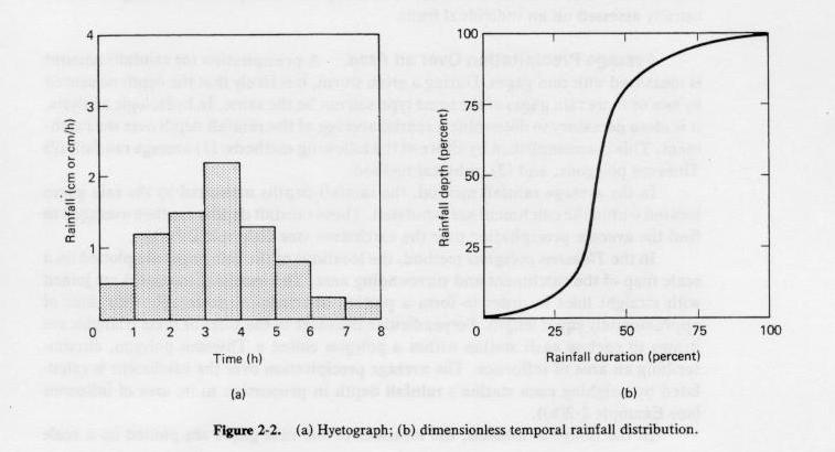
Fig. 2-2

Spatial rainfall distribution

• The same amount of rainfall does not fall uniformly over the entire catchment.

• Isohyets depict the spatial variation of rainfall (Fig. 2-4)

• In regional rainfall maps, isohyets are referred to as isopluvials.

• San Diego County 24-hr isopluvials.

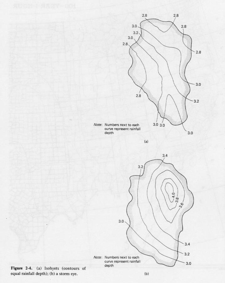
Fig. 2-4

Average precipitation over an area

• It is often necessary to determine a spatial average of precipitation.

• This is performed in three ways:
  
  
  1. Average method: raingage depths are averaged without regard to intensity or areal distribution.

  2. Thiessen polygons: raingage locations are joined with straight lines, and perpendicular bisectors determine the area of influence of each raingage.

  3. Isohyetal method: raingage depths are used to draw contours of equal rainfall (isohyets); mid-distance between two adjacent isohyets determine area of influence of each isohyet.

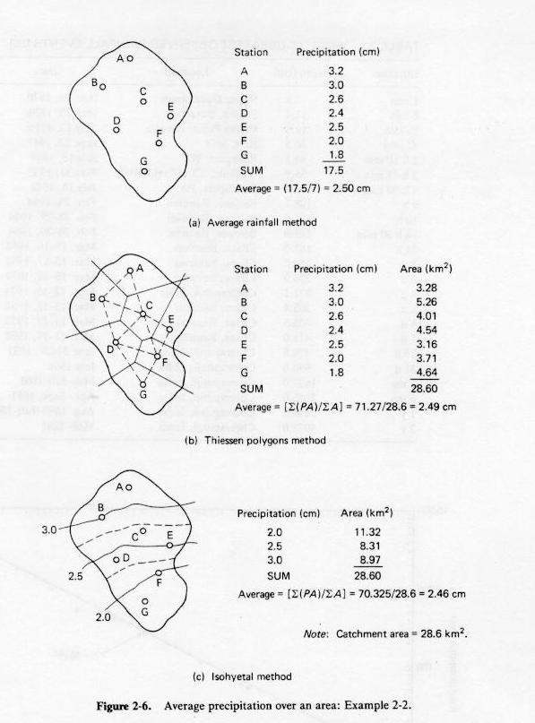
Fig. 2-6

Storm analysis

• Storm depth h and duration t are directly related.

  h = c t n

• Exponent n varies between 0.2 and 0.5.

• Depth-duration data for the world's greatest observed rainfall events.

  h = 39 t 0.5

  Fig. 2-7

• Differentiating rainfall depth with respect to duration:

  dh/dt = i = c n t n-1

• Simplifying:

  i = a / t m

• in which a = cn; and m = 1 - n.

• A more general intensity-duration model is:

  i = a / (t + b) m

• An intensity-duration-frequency model is:

  i = K Tn / (t + b) m

• in which K = a coefficient; and n = an exponent.

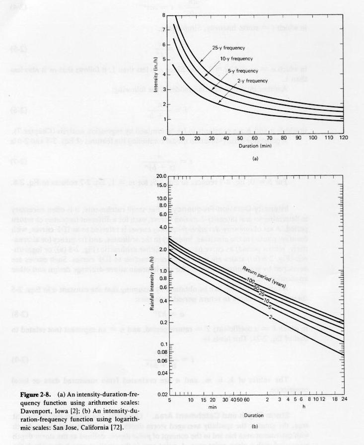
  Fig. 2-8

Storm depth and catchment area

• Generally, the greater the catchment, the smaller the spatially averaged storm depth.

• Point depth is the storm depth associated with a point area.

• Point area is the smallest area below which the variation of storm depth with catchment area is assumed negligible.

• Reduction in point depth is warranted for large catchments.

• NWS depth-area reduction charts are available.

Fig. 2-9

Depth-duration-frequency

• Isopluvial maps depicting storm depths for a range of durations, frequencies, and catchment areas are available for the entire U.S.

• These maps usually show point-depth values.

• San Diego County 24-hr isopluvials.

Depth-area-duration

• This is an alternate way of portraying the reduction of storm depth with area, with duration as a third variable.

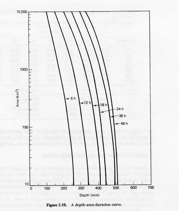
Fig. 2-10

Sources of precipitation data

• NOAA

• National Weather Service NOAA

Filling in missing records

• Incomplete records of rainfall are sometimes due to operation error or equipment malfunction.

• The mean annual rainfall N for stations X, A, B, and C is evaluated.

• If the mean annual rainfall at A, B, and C is within 10% of that of X, a simple average is sufficient.

• If not, then the normal ratio method is used to fill in missing records at station X:

  PX = (1/3) [(NX/NA)PA + (NX/NB)PB + (NX/NC)PC ]

• in which P = precipitation, N = mean annual rainfall, for stations X, A, B, and C.

• In the NWS method, data for four neighboring stations (one in each quadrant) is weighted in proportion to the reciprocal of the square of its distance to station X.

Fig. 2-11

• The procedure is described by the following formula:

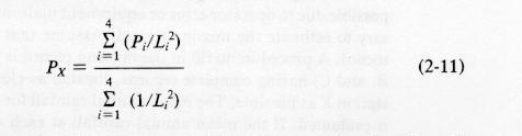
Eq. 2-11

Double-mass analysis

• Consistency of a rainfall record is tested with double-mass analysis.

• This method compares the cumulative annual or seasonal values of station Y with those of a reference station X.

• The reference station X is usually the mean of several neighboring stations.

• The cumulative pairs are plotted in an x-y coordinate system.

• If the plot is linear, the record for Y is consistent.

• If the plot shows a break in slope, the record for station Y is inconsistent.

• Correction is performed by adjusting the records prior to the break to reflect the new state (after the break).

• The rainfall records prior to the break are multiplied by the ratio of slopes after and before the break.

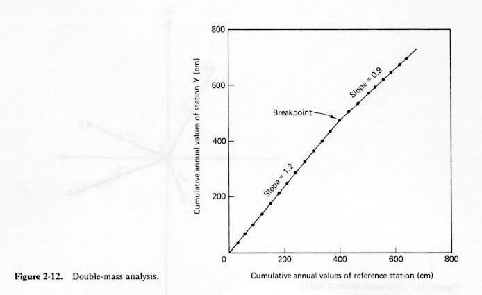
Fig. 2-12

Go to Chapter 2B.