[Equation of Gradually Varied Flow]   [Characteristics of Flow Profiles]   [Limits to Water Surface Profiles]   [Methodologies]   [Direct Step Method Example]   [Questions]   [Problems]   [References]     

CHAPTER 7:
GRADUALLY VARIED FLOW


7.1  EQUATION OF GRADUALLY VARIED FLOW

[Characteristics of Flow Profiles]   [Limits to Water Surface Profiles]   [Methodologies]   [Direct Step Method Example]   [Questions]   [Problems]   [References]      [Top]  

The flow is gradually varied when the discharge Q is constant but the other hydraulic variables (A, V, D, R, P, and so on) vary gradually in space. The basic assumptions of gradually varied flow are:

  1. The flow is steady, i.e., none of the hydraulic variables vary in time.

  2. The streamlines are essentially parallel; thus, the pressure distribution in the vertical direction is hydrostatic, i.e., proportional to the flow depth.

  3. The head loss is the same as that corresponding to uniform flow; therefore, the uniform flow formula may be used to evaluate the energy slope.

  4. The value of Manning's n is the same as that of uniform flow.

Other assumptions of gradually varied flow are:

  1. The slope of the channel is small.

  2. The pressure correction factor cosθ ≅ 1.

  3. There is negligible air entrainment.

  4. The conveyance is an exponential function of the flow depth (except for the case of circular culverts).

  5. The roughness (Manning's n) is independent of the flow depth (only an approximation) and is constant throughout the reach under consideration.

Fig. 7-1  Definition sketch for energy in open-channel flow.

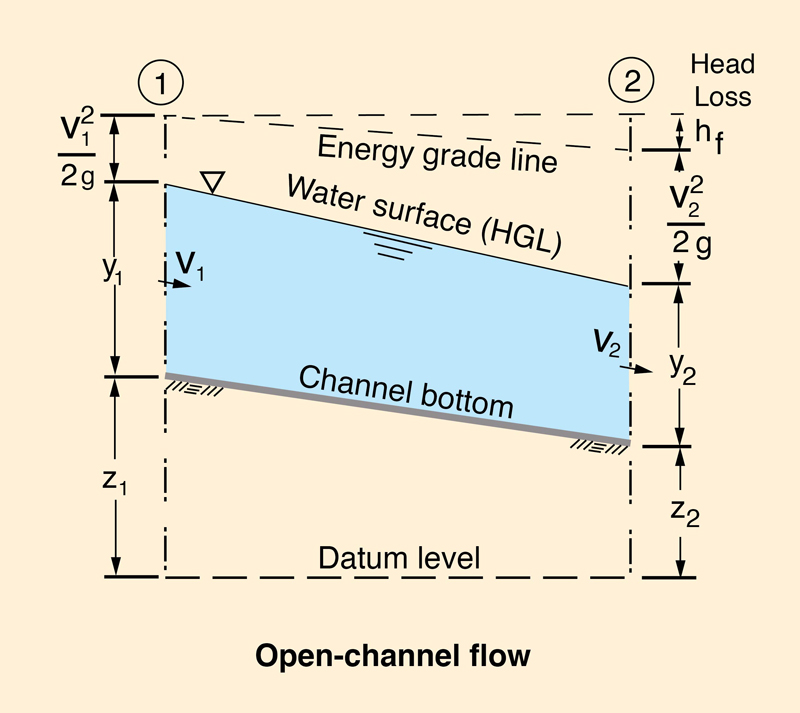
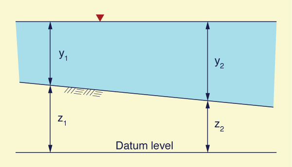
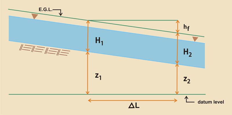
Under gradually varied flow, the gradient of hydraulic head is (Fig. 7-1):

  dH         d                      V 2
_____  =  ___ ( z  +  y  +  _____ )  =  - Sf
  dx         dx                      2g
(7-1)

The negative sign in front of the friction slope Sf is required because the flow direction is from left to right, while the derivative is taken from right to left, by convention. By definition, the friction slope is:

            hf                   
Sf  =  _____
           ΔL                  
(7-2)

in which ΔL = length of the channel reach under consideration.

The gradient of specific energy is:

  dE         d               V 2             dz
_____  =  ___ ( y  +  _____ )  =  - ____  -  Sf
  dx         dx              2g              dx
(7-3)

The gradient of the channel bed, or channel slope (bottom slope), is:

  dz          z2 - z1                    
_____  =  ________
  dx             ΔL                   
(7-4)

      dz          z1 - z2                    
 -  _____  =  ________  =  So
      dx             ΔL                   
(7-5)

Therefore, the gradient of specific energy is:

  dE         d               V 2              
_____  =  ___ ( y  +  _____ )  =  So  -  Sf
  dx         dx              2g              
(7-6)

Under steady flow: Q = V A = constant. Therefore:

  d                 Q 2              
____ ( y  +  _______ )  =  So  -  Sf
 dx              2g A2              
(7-7)

  dy           d           Q 2              
_____  +  _____   ( _______ )  =  So  -  Sf
  dx           dx        2g A2              
(7-8)

  dy            Q 2       dA         
_____  -  ( ______ ) _____  =  So  -  Sf
  dx           g A3       dx        
(7-9)

  dy            Q 2       dA     dy         
_____  -  ( ______ ) _____ _____   =  So  -  Sf
  dx           g A3       dy     dx        
(7-10)

Using Eq. 3-11:

  dy            Q 2 T       dy         
_____  -  ( ________ ) _____   =  So  -  Sf
  dx             g A3        dx        
(7-11)

Therefore, the flow-depth gradient is:

  dy                    So  -  Sf              
_____  =  _______________________
  dx          1  -  [(Q 2 T ) / (g A3)]             
(7-12)

The friction slope based on the Chezy equation (Eqs. 5-10 and 2-4) is:

                 Q 2               
Sf  =  ____________
           C 2 A2 R             
(7-13)

Since R = A / P :

            Q 2 P               
Sf  =  _________
           C 2 A3              
(7-14)

Substituting Eq. 7-14 into Eq. 7-12, the flow-depth gradient is:

  dy           So  -  [(Q 2 P ) / (C 2 A3)]              
_____  =  ___________________________
  dx              1  -  [(Q 2 T ) / (g A3)]             
(7-15)

  dy           So  -  (g/C 2) (P / T ) [(Q 2 T ) / (g A3)]              
_____  =  _______________________________________
  dx                       1  -  [(Q 2 T ) / (g A3)]             
(7-16)

The square of the Froude number is (Eq. 3-12):

              Q 2 T               
F 2  =  _________
               g A3             
(7-17)

Substituting Eq. 7-17 into Eq. 7-16:

  dy           So  -  (g/C 2) (P / T ) F 2              
_____  =  _________________________
  dx                       1  -  F 2             
(7-18)

Substituting Eq. 5-12 into Eq. 7-18:

  dy           So  -  f (P / T ) F 2              
_____  =  _____________________
  dx                    1  -  F 2             
(7-19)

Therefore, the depth gradient (dy/dx) is a function of:

  1. Channel slope So,

  2. Friction coefficient f,

  3. Ratio of wetted perimeter to top width P / T, and

  4. Froude number.

For dy/dx = 0, Eq. 7-19 reduces to a statement of uniform flow:

                            
So  =  f (P / T ) F 2
                                   
(7-20)

For F = 1, Eq. 7-20 reduces to a statement of critical uniform flow:

                            
So  =  f (Pc / Tc )  =  Sc
                                   
(7-21)

in which Sc = critical slope, i.e., the channel slope for which the flow is critical.

In terms of critical slope (Eq. 7-21), the flow-depth gradient is:

  dy           So  -  (P / T ) (Tc / Pc ) Sc F 2              
_____  =  ________________________________
  dx                            1  -  F 2             
(7-22)

For (P / T ) ≅ (Pc / Tc ), i.e., for a constant ratio (P / T) with flow depth, Eq. 7-22 reduces to:

  dy           So  -  Sc F 2              
_____  =  _______________
  dx               1  -  F 2             
(7-23)

For conciseness, the flow-depth gradient can be written as:

            dy                         
Sy  =  _____
            dx                           
(7-24)

Substituting Eq. 7-24 into Eq. 7-23, the flow-depth gradient is:

 Sy           (So / Sc)  -  F 2      
____  =  __________________
 Sc                  1  -  F 2
(7-25)

Equation 7-25 (or 7-23) is the gradually varied flow equation. The depth gradient Sy is a function only of: (1) channel slope So, (2) critical slope Sc, and (3) Froude number F.

Note on the applicability of Eq. 7-25


Strictly speaking, Eq. 7-25 applies only for the case (P / T ) (Tc / Pc ) = 1, which is the same as (P / T ) = (Pc / Tc ); that is, for a constant ratio (P / T ), regardless of flow depth. This condition is less restrictive that the (asymptotic) hydraulically wide channel condition, for which (P / T ) = 1. Therefore, for a hydraulically wide channel, for which PT, it follows that: (P / T ) (Tc / Pc ) ≅ 1. Thus, it is concluded that Eq. 7-25 applies for a hydraulically wide channel.


7.2  CHARACTERISTICS OF FLOW PROFILES

[Limits to Water Surface Profiles]   [Methodologies]   [Direct Step Method Example]   [Questions]   [Problems]   [References]      [Top]   [Equation of Gradually Varied Flow]  

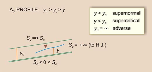
In Eq. 7-25, the sign of the left-hand side (LHS) is that of Sy (numerator), since Sc (denominator) is always positive (friction is always positive). The sign of Sy (i.e, the sign of the LHS) may be one of three possibilities:

  • A positive value, leading to RETARDED FLOW (BACKWATER),

  • A zero value, leading to UNIFORM FLOW (NORMAL), or

  • A negative value, leading to ACCELERATED FLOW (DRAWDOWN).

In the right-hand side (RHS) of Eq. 7-25, there are three possibilities for the numerator (USDA Soil Conservation Service, 1971):

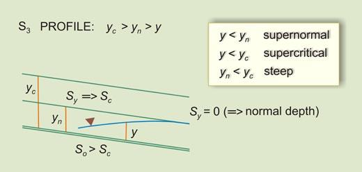
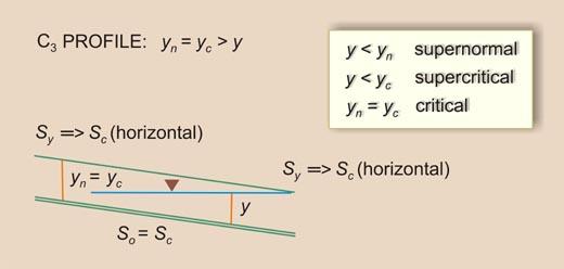
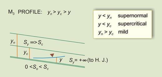
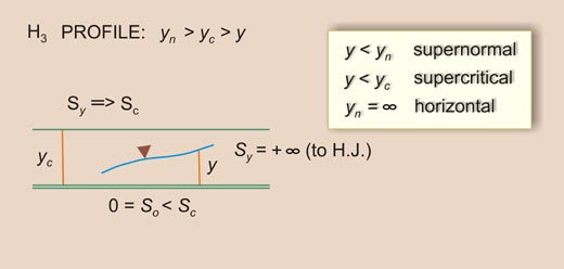
  • So / Sc > F 2, leading to SUBNORMAL FLOW,

  • So / Sc = F 2, leading to NORMAL FLOW, or

  • So / Sc < F 2, leading to SUPERNORMAL FLOW.

There are three possibilities for the denominator:

  • 1 > F 2, leading to SUBCRITICAL FLOW,

  • 1 = F 2, leading to CRITICAL FLOW, or

  • 1 < F 2, leading to SUPERCRITICAL FLOW.

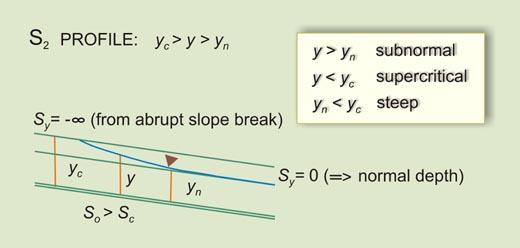
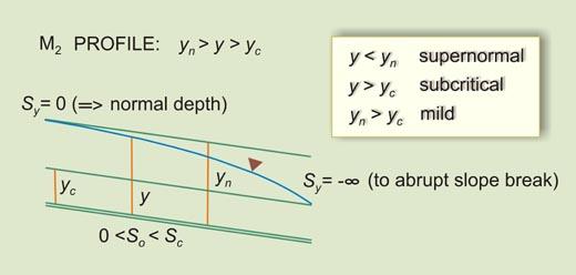
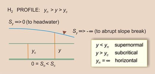
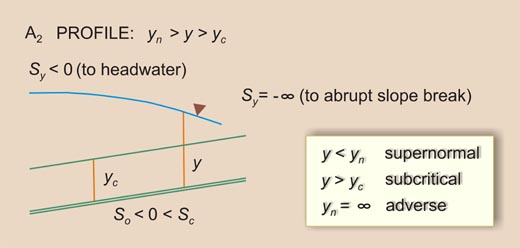
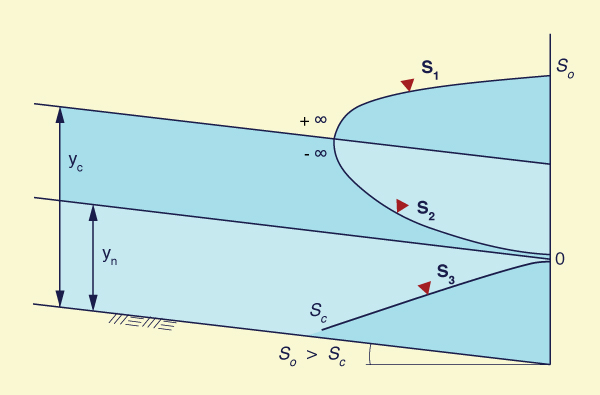
Given the above inequalities, there arise three types (or families) of water-surface profiles, shown in Table 7-1. The total number of profiles is 12. A summary is shown in Table 7-2.

Table 7-1  Types of water-surface profiles.
Type Description Numerator and denominator of RHS
of Eq. 7-25
Sign
of
LHS
Flow
profile
I Subnormal/subcritical flow Both numerator and denominator are positive + Retarded
IIA Subnormal/supercritical flow Numerator is positive and denominator is negative - Accelerated
BSupernormal/subcritical flow Numerator is negative and denominator is positive - Accelerated
IIISupernormal/supercritical flow Both numerator and denominator are negative + Retarded

Table 7-2  Summary of water-surface profiles.
Family Character Rule So > Sc So = Sc So < Sc So = 0 So < 0
I Retarded
(Backwater)
1 > F 2 < (So / Sc) S1 C1 M1 - -
IIA Accelerated
(Drawdown)
1 < F 2 < (So / Sc) S2 - - - -
B Accelerated
(Drawdown)
1 > F 2 > (So / Sc) - - M2 H2 A2
III Retarded
(Backwater)
1 < F 2 > (So / Sc) S3 C3 M3 H3 A3


Type I

In the Type I family, the flow is subnormal/subcritical. Therefore, the rule is:

                            
1  >  F 2  <  (So / Sc )
                                   
(7-26)

which is the same as:

                            
(So / Sc )  > <  1
                                   
(7-27)

Equation 7-27 states that So may be lesser than, equal to, or greater than Sc . This gives rise to three types of profiles:


  • M1:  So < Sc

    Definition sketch for M<sub>1</sub> water-surface profile

    Fig. 7-2  Definition sketch for M1 water-surface profile.

    The depth gradient Sy varies from asymptotic to So (i.e., asymptotic to the horizontal) at the downstream end to asymptotic to zero (i.e., asymptotic to the normal depth) at the upstream end.


  • C1:  So = Sc

    Definition sketch for C<sub>1</sub> water-surface profile

    Fig. 7-3  Definition sketch for C1 water-surface profile.

    The depth gradient Sy varies from Sc at the downstream end to Sc at the upstream end, i.e., the water-surface profile is a horizontal line.


  • S1:  So > Sc

    Definition sketch for S<sub>1</sub> water-surface profile

    Fig. 7-4  Definition sketch for S1 water-surface profile.

    The depth gradient Sy varies from asymptotic to So (i.e., asymptotic to the horizontal) at the downstream end to asymptotic to + ∞ (i.e., asymptotic to the hydraulic jump) at the upstream end.


Since
                            
(So / Sc )  >  F 2
                                   
(7-28)

and

                            
F 2  >  0
                                   
(7-29)

it follows that
                            
(So / Sc )  >  0
                                   
(7-30)

Thus:
                            
So  >  0
                                   
(7-31)

Therefore, no horizontal (H) or adverse (A) profiles are possible in the Type I family of water-surface profiles.


Type II A

In the Type II A family, the flow is subnormal/supercritical. Therefore, the rule is:

                            
1  <  F 2  <  (So / Sc )
                                   
(7-32)

which is the same as:

                            
(So / Sc )  >  1
                                   
(7-33)

Equation 7-33 states that So may only be greater than Sc . This gives rise to only one profile:


  • S2:  So > Sc

    Definition sketch for S<sub>2</sub> water-surface profile

    Fig. 7-5  Definition sketch for S2 water-surface profile.

    The depth gradient Sy varies from - ∞ (i.e., asymptotic to an abrupt slope break) at the upstream end to asymptotic to zero (i.e., asymptotic to the normal depth) at the downstream end.


Since
                            
(So / Sc )  >  F 2
                                   
(7-34)

and

                            
F 2  >  0
                                   
(7-35)

it follows that

                            
(So / Sc )  >  0
                                   
(7-36)

Thus:
                            
So  >  0
                                   
(7-37)

Therefore, no horizontal (H) or adverse (A) profiles are possible in the Type II A family of water-surface profiles.


Type II B

In the Type II B family, the flow is supernormal/subcritical. Therefore, the rule is:

                            
1  >  F 2  >  (So / Sc )
                                   
(7-38)

which is the same as:

                            
(So / Sc )  <  1
                                   
(7-39)

Equation 7-39 states that So may be lesser than Sc , equal to 0, or lesser than 0. This gives rise to three types of profiles:


  • M2:  0 <  So < Sc

    Definition sketch for M<sub>2</sub> water-surface profile

    Fig. 7-6  Definition sketch for M2 water-surface profile.

    The depth gradient Sy varies from - ∞ (i.e., abrupt slope break) at the downstream end to asymptotic to zero (i.e., asymptotic to the normal depth) at the upstream end.


  • H2: 0 =  So < Sc

    Definition sketch for H<sub>2</sub> water-surface profile

    Fig. 7-7  Definition sketch for H2 water-surface profile.

    The depth gradient Sy varies from - ∞ (i.e., abrupt slope break) at the downstream end to asymptotic to 0 (to headwater) at the upstream end.


  • A2:  So < 0 < Sc

    Definition sketch for A<sub>2</sub> water-surface profile

    Fig. 7-8  Definition sketch for A2 water-surface profile.

    The depth gradient Sy varies from - ∞ (i.e., abrupt slope break) at the downstream end to asymptotic to < 0 (to headwater) at the upstream end.


Type III

In the Type III family, the flow is supernormal/supercritical. Therefore, the rule is:

                            
1  <  F 2  >  (So / Sc )
                                   
(7-44)

which is the same as:

                            
(So / Sc )  > <  1
                                   
(7-45)

Equation 7-45 states that So may be lesser than, equal to, or greater than Sc . This gives rise to five types of profiles:


  • S3:  So > Sc

    Definition sketch for S<sub>3</sub> water-surface profile

    Fig. 7-9  Definition sketch for S3 water-surface profile.

    The depth gradient Sy varies from asymptotic to Sc at the upstream end to asymptotic to zero (i.e., asymptotic to the normal depth) at the downstream end.


  • C3:  So = Sc

    Definition sketch for C<sub>3</sub> water-surface profile

    Fig. 7-10  Definition sketch for C3 water-surface profile.

    The depth gradient Sy varies from Sc at the downstream end to Sc at the upstream end, i.e., the water-surface profile is a horizontal line.


  • M3:  0 <  So < Sc

    Definition sketch for M<sub>3</sub> water-surface profile

    Fig. 7-11  Definition sketch for M3 water-surface profile.

    The depth gradient Sy varies from asymptotic to Sc at the upstream end to asymptotic to + ∞ (i.e., asymptotic to the hydraulic jump) at the downstream end.


  • H3:  0 =  So < Sc

    Definition sketch for H<sub>3</sub> water-surface profile

    Fig. 7-12  Definition sketch for H3 water-surface profile.

    The depth gradient Sy varies from asymptotic to Sc at the upstream end to asymptotic to + ∞ (i.e., asymptotic to the hydraulic jump) at the downstream end.


  • A3:  So = Sc

    Definition sketch for A<sub>3</sub> water-surface profile

    Fig. 7-13  Definition sketch for A3 water-surface profile.

    The depth gradient Sy varies from asymptotic to Sc at the upstream end to asymptotic to + ∞ (i.e., asymptotic to the hydraulic jump) at the downstream end.


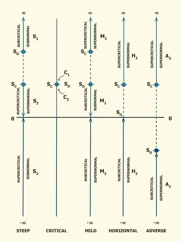
Figure 7-14 shows a graphical representation of flow-depth gradients in water-surface profile computations. The arrows indicate the direction of computation.

Definition sketch for A<sub>3</sub> water-surface profile

Fig. 7-14  Graphical representation of flow-depth gradient ranges
in water-surface profile computations.


7.3  LIMITS TO WATER SURFACE PROFILES

[Methodologies]   [Direct Step Method Example]   [Questions]   [Problems]   [References]      [Top]   [Equation of Gradually Varied Flow]   [Characteristics of Flow Profiles]  

The flow-depth gradients vary between five (5) limits (Fig. 7-14):

  1. The channel slope So

  2. The critical slope Sc

  3. Zero.

  4. + ∞

  5. - ∞

The theoretical limits to the water-surface profiles may be analyzed using Eq. 7-25, repeated here in a slightly different form:

             So  -  Sc F 2      
Sy  =  ______________
               1  -  F 2
(7-46)

Operating in Eq. 7-46:

                   
Sy (1  -  F 2)  =  So  -  Sc F 2
               
(7-47)

             So  -  Sy      
F 2  =  ____________
             Sc  -  Sy
(7-48)

For uniform (normal) flow: Sy  =  0, and Eq. 7-48 reduces to:
                   
So  =  Sc F 2
               
(7-49)

For gradually varied flow: Sy  ≠  0, and Eq. 7-48 is subject to three (3) cases:

  • ONE

    F 2 > 0

    • So > Sy  and  Sc > Sy

      The following inequality is satisfied: So > Sy < Sc

    • So < Sy  and  Sc < Sy

      The following inequality is satisfied: So < Sy > Sc

    • It is concluded that Sy has to be either less than both So and Sc, or greater than both.

  • TWO

    F 2 = 0

    This leads to:  So = Sy

                z1 - z2      
    So  =  _________
                    L
    (7-51)

                y2 - y1      
    Sy  =  _________
                    L
    (7-52)

    Combining Eqs. 7-51 and 7-52:

                      
    z1 + y1  =  z2 + y2
                    
    (7-53)

    Equation 7-53 depicts a true reservoir (Fig. 7-15).

    True reservoir condition.

    Fig. 7-15  True reservoir condition.

  1. THREE

    F 2 < 0:  Since F ≥ 0, this condition is impossible.

    The following inequality is NOT satisfied:  So > Sy > Sc

    The following inequality is NOT satisfied:  So < Sy < Sc

    It is concluded that Sy cannot be less than So and greater than Sc , or less than Sc and greater than So . Thus, Sy has to be less than both So AND Sc, or greater than both (See Case 1).


Uses of water-surface profiles

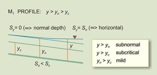
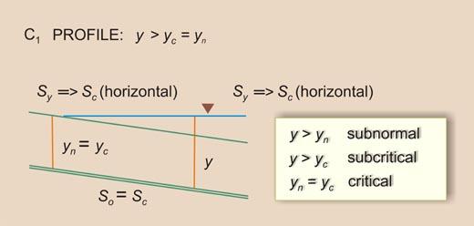
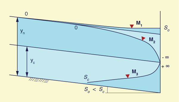
Table 7-3 and Fig. 7-16 show the typical occurrence of mild water-surface profiles.

Table 7-3  Occurrence of mild water-surface profiles.
M1 Flow in a mild channel, upstream of a reservoir.
M2 Flow in a mild channel, upstream of an abrupt change in grade or a steep channel carrying supercritical flow.
M3 Flow in a mild channel, downstream of a steep channel carrying supercritical flow.

Typical occurrence of mild profiles.

Fig. 7-16  Typical occurrence of mild profiles.

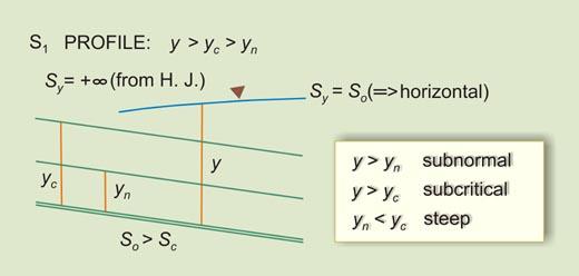
Table 7-4 and Fig. 7-17 show the typical occurrence of steep water-surface profiles.

Table 7-4  Occurrence of steep water-surface profiles.
S1 Flow in a steep channel, upstream of a reservoir.
S2 Flow in a steep channel, downstream of a mild channel carrying subcritical flow.
S3 Flow in a steep channel, downstream of a steeper channel carrying supercritical flow.

Typical occurrence of steep profiles.

Fig. 7-17  Typical occurrence of steep profiles.


7.4  METHODOLOGIES

[Direct Step Method Example]   [Questions]   [Problems]   [References]      [Top]   [Equation of Gradually Varied Flow]   [Characteristics of Flow Profiles]   [Limits to Water Surface Profiles]  

There are two ways to calculate water-surface profiles:

  1. The direct step method.

  2. The standard step method.

The direct step method is applicable to prismatic channels, while the standard step method is applicable to any channel, prismatic and nonprismatic (Table 7-5). The direct step method is direct, readily amenable to use with a spreadsheet, and relatively straight forward in its solution. The standard step method is iterative and complex in its solution. In practice, the standard step method is represented by the Hydrologic Engineering Center's River Analysis System, referred to as HEC-RAS (U.S. Army Corps of Engineers, 2014).

The direct step method applies particularly where data is scarce and resources are limited. The standard step method applies for comprehensive projects. The use of a widely accepted government program such as HEC-RAS enhances credibility.

The required number of cross sections in the standard step method increases with the channel slope. Steeper channels may require more cross sections. Lesser cross sectional variability results in more reliable and accurate results. Note that extensive two- and three-dimensional flow features may not be accurately represented in the one-dimensional water-surface profile model.

Table 7-5  Comparison between direct step and standard step methods.
No. CharacteristicDirect step method Standard step method
1 Cross-sectional shapePrismatic Any (prismatic or nonprismatic)
2 Ease of computationEasy (hours) Difficult (months)
3Calculation advances ⇒ Directly By iteration (trial and error)
4 Type of cross-section inputOne typical cross section (prismatic) Several cross sections (nonprismatic)
5 Data needsMinimal Extensive
6Accuracy increases with ↠A smaller flow depth increment More cross sections and/or lesser cross-sectional variability
7 Independent variableFlow depth Length of channel
8 Dependent variableLength of channel Flow depth
9 ToolsSpreadsheet or programming HEC-RAS
10 ReliabilityAnswer is always possible Answer is sometimes not possible, depending on the type of cross-sectional input data
11 CostComparatively small Comparatively large
12 Public acceptanceAverage High


7.5  DIRECT STEP METHOD EXAMPLE

[Questions]   [Problems]   [References]      [Top]   [Equation of Gradually Varied Flow]   [Characteristics of Flow Profiles]   [Limits to Water Surface Profiles]   [Methodologies]  

Calculation of M2 and S2 profiles, upstream and downstream of a change in grade, from mild to steep

Definition sketch for M<sub>2</sub> water-surface profile
Definition sketch for S<sub>2</sub> water-surface profile

Input data:

  • Discharge Q = 2000 m3

  • Bottom width b = 100 m.

  • Side slope 2 H : 1 V

  • Upstream channel slope = 0.0001

  • Upstream channel Manning's n = 0.025

  • Downstream channel slope = 0.03

  • Downstream channel Manning's n = 0.045

Solution

Calculate the normal depth and velocity, and critical depth and velocity, in the upstream and downstream channels. Use ONLINE CHANNEL 05.

For the upstream channel:

  • Normal depth = 10.098 m

  • Normal velocity = 1.648 m/s

  • Normal Froude number = 0.179

  • Critical depth = 3.364 m

  • Critical velocity = 5.571 m/s

    For the downstream channel:

  • Normal depth = 2.669 m

  • Normal velocity = 7.113 m/s

  • Normal Froude number = 1.425

  • Critical depth = 3.364 m

  • Critical velocity = 5.571 m/s

    Calculation of critical slope for the upstream channel:

  • yc = 3.364 m

  • Vc = 5.571 m/s

  • Ac = (b + zyc ) yc = 359.033 m2

  • P = b + 2 yc (1 + z 2)1/2 = 115.044 m

  • Rc = Ac / Pc = 3.121 m

  • Sc = n 2 Vc2 / Rc4/3 = (0.025)2 (5.571)2 (3.121)4/3 = 0.00425

  • Verify the critical slope with ONLINE CHANNEL 04:  Sc = 0.004254.

    Calculation of critical slope for the downstream channel:

  • Sc = n 2 Vc2 / Rc4/3 = (0.045)2 (5.571)2 (3.121)4/3 = 0.0138

  • Verify the critical slope with ONLINE CHANNEL 04:  Sc = 0.01378.

    The calculation of the M2 water-surface profile is shown in Table 7-6. The following instructions are indicated:

  • The calculation moves in the upstream direction, starting at critical depth at the downstream end.

  • Column [1]:  The second depth is set at 4 m; subsequently, the depth interval is set at 1 m.

  • Column [2]:  The flow area is:  A = (b + zy ) y                     . . . (1)

  • Column [3]:  The mean velocity is:  V = Q / A                     . . . (2)

  • Column [4]:  The velocity head is:  V 2 / (2g)                     . . . (3)

  • Column [5]:  The specific head is:  H = y + V 2 / (2g)                     . . . (4)

  • Column [6]:  The wetted perimeter is:  P = b + 2 y (1 + z 2)1/2                     . . . (5)

  • Column [7]:  The hydraulic radius is:  R = A / P                     . . . (6)

  • Column [8]:  The friction slope is:  Sf = n 2 V 2 / R 4/3                     . . . (7)

  • Column [9]:  The average friction slope is:  Sf ave = 0.5 (Sf 1 + Sf 2)                     . . . (8)

  • Column [10]:  The specific head difference is:  ΔH = H2 - H1                     . . . (9)

  • Column [11]:  The channel length increment ΔL, explained in the box below.

  • Column [12]:  The cumulative channel length, i.e., the cumulative sum of ΔL increments.

    Derivation of the formula for the channel length increment ΔL


    With reference to Fig. 7-18, the average friction slope is:

                      hf      
    Sf ave  =  ______
                      ΔL
    (7-54)

    Definition sketch for the calculation of channel length increment Δ<i>L</i>

    Fig. 7-18  Definition sketch for the calculation of channel length increment ΔL.

                      
    H1 + z1  =  H2 + z2  +  Sf ave ΔL
                    
    (7-55)

                      
    z1 - z2  =  H2 - H1  +  Sf ave ΔL
                    
    (7-56)

                      
    z1 - z2  -  Sf ave ΔL  =  H2 - H1
                    
    (7-57)

                z1 - z2      
    So  =  _________
                   ΔL
    (7-58)

                      
    So ΔL  -  Sf ave ΔL  =  H2 - H1
                    
    (7-59)

                      
    (So  -  Sf ave) ΔL  =  H2 - H1
                    
    (7-60)

                     H2 - H1      
    ΔL  =  ______________
                 So  -  Sf ave
    (7-61)

                        ΔH      
    ΔL  =  ______________
                 So  -  Sf ave
    (7-62)

    Equation 7-62 enables the calculation of the channel length increment ΔL, i.e., Col. 11 of Table 7-6. When ΔL is negative, the calculation moves upstream, as in the M2 profile (Table 7-6). Conversely, when ΔL is positive, the calculation moves downstream, as in the S2 profile (Table 7-7).


    Table 7-6  Calculation of M2 water-surface profile (So = 0.0001).
    [1] [2] [3] [4] [5] [6] [7] [8] [9] [10] [11] [12]
    y A V V 2/(2g ) H P R Sf Sf ave ΔH ΔL ∑ ΔL
      (1) (2) (3) (4) (5) (6) (7) (8) (9) Box  
    3.364 359.033 5.570 1.581 4.945 115.044 3.1208 0.00425 --- --- --- 0
    4.000 432.000 4.630 1.092 5.092 117.888 3.664 0.00237 0.00331 0.147 -45.794 -45.794
    5.000 550.000 3.636 0.674 5.674 122.360 4.495 0.00111 0.00174 0.528 -354.878 -400.672
    6.000 672.000 2.976 0.451 6.451 126.833 5.298 0.00060 0.000855 0.777 -1029.139 -1429.811
    7.000
    8.000
    9.000
    10.000
    10.097 0.0001

    In the direct step method, the accuracy of the computation depends on the size of depth interval (Col. [1] of Table 7-6). The smaller the interval, the more accurate the computation will be. This is because the average friction slope for a subreach (Col. [9]) is the arithmetic average of the friction slopes at the grid points (linear assumption). In practice, a computation using a computer would have a much finer interval than that shown in Table 7-6.

    The calculation of the S2 water-surface profile is shown in Table 7-7.

    Table 7-7  Calculation of S2 water-surface profile (So = 0.03).
    [1] [2] [3] [4] [5] [6] [7] [8] [9] [10] [11] [12]
    y A V V 2/(2g ) H P R Sf Sf ave ΔH ΔL ∑ ΔL
      (1) (2) (3) (4) (5) (6) (7) (8) (9) Box  
    3.364 359.033 5.570 1.581 4.945 115.044 3.1208 0.00425 --- --- --- 0
    3.300 351.780 5.685 1.647 4.9475 114.758 3.0654 0.0147 0.01425 0.002 0.127 0.127
    3.200 340.48 5.874 1.759 4.9586 114.311 2.979 0.0163 0.0155 0.0111 0.765 0.892
    3.100 329.22 6.075 1.881 4.981 113.864 2.891 0.0181 0.0172 0.0224 1.750 2.642
    3.000
    2.900
    2.800
    2.700
    2.669 0.03

    Online calculations

    The M2 water-surface profiles may be calculated online using ONLINE_WSPROFILES_22. Using the number of computational intervals n = 100, and number of tabular output intervals m = 100, the length of the M2 water-surface profile is calculated to be:   ∑ ΔL = 147,691.5 m.

    Definition sketch for M<sub>2</sub> water-surface profile

    Fig. 7-19  Definition sketch for M2 water-surface profile.

    The S2 water-surface profiles may be calculated online using ONLINE_WSPROFILES_25. Using the number of computational intervals n = 100, and number of tabular output intervals m = 100, the length of the S2 water-surface profile is calculated to be:   ∑ ΔL = 152.02 m.

    Definition sketch for S<sub>2</sub> water-surface profile

    Fig. 7-20  Definition sketch for S2 water-surface profile.


    QUESTIONS

    [Problems]   [References]      [Top]   [Equation of Gradually Varied Flow]   [Characteristics of Flow Profiles]   [Limits to Water Surface Profiles]   [Methodologies]   [Direct Step Method Example]  


    PROBLEMS

    [References]      [Top]   [Equation of Gradually Varied Flow]   [Characteristics of Flow Profiles]   [Limits to Water Surface Profiles]   [Methodologies]   [Direct Step Method Example]   [Questions]  


    REFERENCES

       [Top]   [Equation of Gradually Varied Flow]   [Characteristics of Flow Profiles]   [Limits to Water Surface Profiles]   [Methodologies]   [Direct Step Method Example]   [Questions]   [Problems]  

    Chow, V. T. 1959. Open-channel Hydraulics. McGraw Hill, New York.

    U.S. Army Corps of Engineers. (2014). HEC-RAS: Hydrologic Engineering Center River Analysis System.

    USDA Soil Conservation Service. (1971). Classification system for varied flow in prismatic channels. Technical Release No. 47 (TR-47), Washington, D.C.


    http://openchannelhydraulics.sdsu.edu
    140810 18:50
  • Documents in Portable Document Format (PDF) require Adobe Acrobat Reader 5.0 or higher to view; download Adobe Acrobat Reader.