|
|
|
CHAPTER 10: CASCADE ROUTING |
|
"We give a mathematical treatment of the 'competition' between kinematic and dynamic waves in river flow, in order to show how completely the dynamic waves are subordinated in the case of greatest interest, that is, when the speed of the river is well below critical." M. J. Lighthill and G. B. Whitham (1955) |
|
This chapter is divided into six sections. Section 10.1 describes the time-area method of hydrologic catchment routing. Section 10.2 describes the Clark unit hydrograph, a procedure closely related to the time-area method. Section 10.3 deals with the cascade of linear reservoirs, a widely accepted method of hydrologic catchment routing. Sections 10.4 and 10.5 describe two hydraulic methods of catchment routing, based on kinematic and diffusion waves, respectively. Section 10.6 contains a discussion of the capabilities and limitations of catchment routing techniques. |
10.1 TIME-AREA METHOD
|
|
Catchment Routing
Catchment routing refers to the calculation of flows in time and space within a catchment. The objective of catchment routing is to transform effective rainfall into streamflow. This is accomplished either in a lumped mode (e.g., time-area method) or in a distributed mode (e.g., kinematic wave method).
Methods for catchment routing are similar to those of reservoir and stream channel routing. In fact, many techniques used in reservoir and channel routing are also applicable to catchment routing. For instance, the concept of linear reservoir is used in both reservoir and catchment routing. Kinematic wave techniques were originaIl developed for river routing [9], but later were applied to catchment routing [20, 23].
Methods for catchment routing are of two types: (1) hydrologic and (2) hydraulic. Hydrologic methods are based on the storage concept and are spatially lumped to provide a runoff hydrograph at the catchment outlet. Examples of hydrologic catchment routing methods are the time-area method and the cascade of linear reservoirs. Hydraulic methods use kinematic or diffusion waves to simulate surface runoff within a catchment in a distributed context. Unlike hydrologic methods, hydraulic methods can provide runoff hydrographs inside the catchment.
Catchment routing models can use parametric, conceptual, andlor deterministic components. For instance, the hydrograph obtained by the time-area method can be routed through a linear reservoir using a storage constant derived by empirical (i.e., parametric) means. The cascade of linear reservoirs is a typical example of a conceptual model used in catchment routing. Kinematic and diffusion models are examples of deterministic methods used in catchment routing.
The concepts of translation and storage are central to the study of flow routing, whether in catchments, reservoirs, or stream channels. They are particularly important in catchment routing because they can be studied separately, unlike in reservoir and channel routing. Translation may be interpreted as the movement of water in a direction parallel to the channel bottom. Storage may be interpreted as the movement of water in a direction perpendicular to the channel bottom. Translation is synonymous with runoff concentration; storage is synonymous with runoff diffusion.
In reservoir routing, storage is the primary mechanism, with translation almost nonexistent. In stream channel routing, the situation is reversed, with translation being the predominant mechanism and storage playing only a minor role. This. is the reason why kinematic and diffusion waves are useful models of stream channel routing. In catchment routing, translation and storage are about equally important, and, therefore, they are often accounted for separately. The translation effect can be related to runoff concentration, whereas the storage effect can be simulated with linear reservoirs.
Time-Area Method
The time-area method of hydrologic catchment routing transforms an effective storm hyetograph into a runoff hydrograph. The method accounts for translation only and does not include storage. Therefore, hydrographs calculated with the time-area method show a lack of diffusion, resulting in higher peaks than those that would have been obtained if storage had been taken into account. If necessary, the required amount of storage can be incorporated by routing the hydrograph obtained by the time-area method through a linear reservoir. The required amount of storage is determined by calibrating the linear reservoir storage constant K with measured data. Alternatively, suitable values of K can be estimated based on regionally derived formulas.
The time-area method is essentially an extension of the runoff concentration principle used in the rational method (Chapter 4). Unlike the rational method, however, the time-area method can account for the temporal variation of rainfall intensity. Therefore, the applicability of the time-area method is extended to midsize catchments.
The time-area method is based on the concept of time-area histogram, i.e., a histogram of contributing catchment subareas. To develop a time-area histogram, the catchment's time of concentration is divided into a number of equal time intervals. Cumulative time at the end of each time interval is used to divide the catchment into zones delimited by isochrone lines, i.e., the loci of points of equal travel time to the catchment outlet, as shown in Fig. 10-1 (a). For any point inside the catchment, the travel time refers to the time that it would take a parcel of water to travel from that point to the outlet. The catchment subareas delimited by the isochrones are measured and plotted in histogram form as shown in Fig. 10-1 (b).
Figure 10-1 Time-area method: (a) Isochrone delineation; (b) Time-area histogram. |
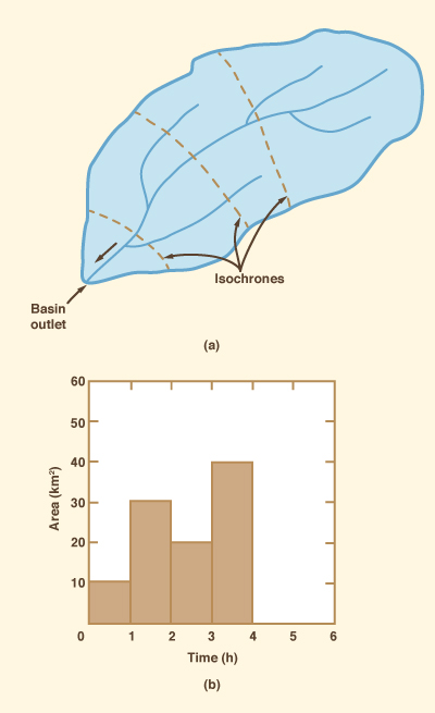
The time interval of the effective rainfall hyetograph should be equal to the time interval of the time-area histogram. The rationale of the time-area method is that, according to the runoff concentration principle (Section 2.4), the partial flow at the end of each time interval is equal to the product of effective rainfall times contributing subarea. The lagging and summation of the partial flows results in a runoff hydrograph for the given effective rainfall hyetograph and time-area histogram. While the time-area method accounts for runoff concentration only, it has the advantage that the catchment shape is reflected in the time-area histogram and, therefore, in the runoff hydrograph. The procedure is illustrated by the following example.
Example 10-1.
A 100-km2 catchment has a 4-h time of concentration, with isochrones at 1-h intervals resulting in the
time-area histogram shown in Fig. 10-1 (b).
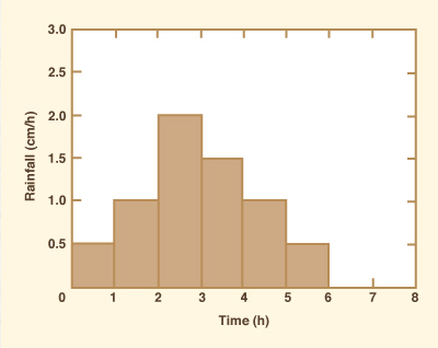
A 6-h storm has the following effective rainfall hyetograph
Figure 10-2 Effective rainfall hyetograph: Example 10-1.
Use the time-area method to calculate the outflow hydrograph.
The routing is shown in Table l0-1.
Column 1 shows time in hours.
The flows shown in Cols. 2-7 were obtained by multiplying effective rainfall intensity times the confributing
partial area.
For instance, Col. 2 shows the contribution of the first effective rainfall interval (0.5 cm/h) on each of the
subareas (10, 30, 20, and 40 km2).
At t = 1 h, the partial flow due to the first effective rainfall interval is 0.5 cm/h × 10 km2 =
5 km2-cm/h (i.e., the flow contributed by the subarea enclosed within the catchment outlet and the first
isochrone takes 1 h to concentrate).
Likewise, at t = 2 h, the partial flow due to the first effective rainfall interval is 0.5 cm/hr × 30 km2 =
The remaining values in Col. 2 (10 and 20) are calculated in a similar way.
Finally, at t = 5 h, the flow is zero because it takes a full time interval (in the absence of runoff diffusion)
for the last concentrated partial flow to recede back to zero.
Columns 2 to 7 show the partial flows contributed by the six effective rainfall intervals, each appropriately lagged a
time interval (because the contribution of the second rainfall interval starts at The sum of these partial flows, shown in Col. 8, is the catchment outflow hydrograph.
In Col. 9, the hydrograph of Col. 8 is expressed in cubic meters per second (Col. 8 × 2.78).
The time base of the outflow hydrograph is 10 h, which is equal to the time of
concentration (4 h) plus the effective
rainfall duration (6 h).
To verify the accuracy of the computations, the sum of Col. 8 is 650 km2-cm/ h, which represents 6.5 cm
of effective rainfall depth uniformly distributed over the entire catchment area (100 km2).
This value (6.5 cm) agrees with the total amount of effective rainfall.
| ||||||||||||||||||||||||||||||||||||||||||||||||||||||||||||||||||||||||||||||||||||||||||||||||||||||||||||||||||||||||||||||||||||||||||||||||||||||||||||||||||||||
It is readily seen that the time-area method and the rational method share a common theoretical basis. However, since the time-area method uses effective rainfall and does not rely on runoff coefficients, it can account only for runoff concentration, with no provision for runoff diffusion. Diffusion can be provided by routing the hydrograph calculated by the time-area method through a linear reservoir with an appropriate storage constant.
The time-area method leads to an alternate way of calculating time of concentration. Provided there is no runoff diffusion as would be the case of a hydrograph calculated by the time-area method, time of concentration can be calculated as the difference between hydrograph time base and effective rainfall duration. Intuitively, as rainfall ceases, the farthest parcels of water concentrate at the catchment outlet at a time equal to the time of concentration. Therefore:
| tc = Tb - tr | (10-1) |
in which tc = time of concentration, Tb = time base of the translated-only hydrograph, and tr = effective rainfall duration.
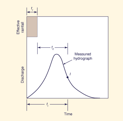
Equation 10-1 can also be expressed in a slightly different form. Assuming that the point of inflection (i.e., the point of zero curvature) on the receding limb of a measured (i.e., translated and diffused) hydrograph coincides with the end of the translated-only hydrograph, the time to point of inflection of the measured hydrograph can be used in Eq. 10-1 in lieu of time base. Therefore time of concentration can be defined as the difference between the time to point of inflection and the effective rainfall duration (see Fig. 10-3):
| tc = ti - tr | (10-2) |
in which ti = time to point of inflection on the receding limb of a measured hydrograph. The advantage of Eq. 10-2 over Eq. 10-1 is that, unlike the time base of the translated-only hydrograph, the point of inflection on the receding limb of a measured hydrograph can be readily ascertained.
Figure 10-3 Alternate definition of time of concentration. |
10.2 CLARK UNIT HYDROGRAPH
|
|
The procedure to derive a Clark unit hydrograph parallels that of the time-area method [2]. First, it is necessary to determine the catchment isochrones. In the Clark method, however, a unit effective rainfall is used in lieu of the effective storm hyetograph used in the time-area method. This leads to an outflow hydrograph corresponding to a unit runoff depth, that is, a unit hydrograph. Since the unit hydrograph calculated in this way lacks runoff diffusion, Clark suggested that it be routed through a linear reservoir. As with the time-area method, an estimate of the linear reservoir storage constant is required. This can be obtained either from the tail� of a measured hydrograph or by using a regionally derived formula. In the latter case, the Clark unit hydrograph can be properly regarded as a synthetic unit hydrograph.
Like the time-area method, the Clark unit hydrograph method has the advantage that the catchment's properties (shape, hydraulic length, surface roughness, and so on) are reflected in the time-area histogram and, therefore, on the shape of the unit hydrograph. This feature has contributed to the popularity of the Clark unit hydrograph in engineering practice [7].
When using the Clark or time-area methods, the storage constant can be estimated from the tail of a measured hydrograph. For this purpose, the differential equation of storage (Eq. 8-4) is evaluated at a time for which inflow equals zero (I = 0), i.e., past the end of the translated-only hydrograph. Alternatively, it can be evaluated at the point of inflection on the receding limb of a measured hydrograph (Fig. 10-3). This leads to:
| (10-3) |
and since S = KO, the following expression for K is obtained:
| (10-4) |
in which O and dO / dt are evaluated past the end of the translated-only hydrograph or at (the time to) the point of inflection on the receding limb of a measured hydrograph.
The derivation of the Clark unit hydrograph is illustrated by the following example.
Example 10-2.
Use the Clark method to derive a 2-h unit hydrograph for the catchment of Example 10-1.
To provide storage, route the translated-only hydrograph through a linear reservoir of storage constant K = 2 h.
Use Δt = 1 h.
The 2-h unit hydrograph has an effective rainfall intensity of 0.5 cm/ h (i.e. , 1-cm depth over a 2�h duration).
The calculations are shown in Table 10-2.
Column 1 shows time in
hours.
Column 2 shows the contribution of the first hour, with 0.5 cm/h of effective rainfall.
The procedure is the same as in Table 10-1 , Cal. 2.
Column 3 shows the contribution of the second hour, with 0.5 cm/ h of effective rainfall.
Again, the procedure is the same as in Tabie 10-1, Col. 2; but the partial flows are lagged 1 h.
The translated-only unit hydrograph shown in Col. 4 is the sum of the partial flows (Cols. 2 and 3).
The translated-only unit hydrograph (Col. 4) is the inflow to the linear reservoir.
With Δt/K = 1/2, the routing coefficients (Table 8-1) are C0 = 1/5, C1 = 1/5, and C2 = 3/5.
The partial flows of the linear reservoir routing are shown in Cols. 5 to 7, and the translated-and-diffused unit hydrograph (in km2*cm/h) shown in Col. 8 is the sum of Cols. 5 to 7 (See Example 8-1 for details of the linear reservoir-routing procedure).
Column 9 shows the trarislated-anddiffused Clark unit hydrograph in cubic meters per second.
The sum of the ordinates of the translated-only hydrograph (Col. 4) is 100, which amounts to 1 cm of effective rainfall depth uniformly distributed over 100 km2 of catchment area.
Likewise, the sum of the ordinates of the translated-and-diffused hydrograph (Col. 8) is 99.98, which verifies not only that the calculated hydrograph is a unit hydrograph but also that the calculation is mass (i.e., volume) conservative.
Notice that the peak of the translated-only unit hydrograph (Col. 4) is 30 km2*cm/ h, whereas the peak of the translated-and-diffused unit hydrograph (Col. 8) is 21.05 km2*cm/ h.
Also, notice that the time bilse of the translatedonly unit hydrograph ends sharply at 6 h, whereas the time base of the translated and diffused unit hydrograph is much longer, with the receding limb of the unit hydrograph gradually approaching zero.
This reveals the substantial amount of r!lnoff diffusion provided by the linear reservoir.
Note that in the Clark method, the number of partial flows (2 in Example 10-2 shown as Cols. 2 and 3 of Table 10-2) is equal to the duration of the unit hydrograph (2 h) divided by the (chosen) time interval of histogram definition (1 h).
Also, the unit effective rainfall intensity (0.5 cm/h) is equal to the unit rainfall depth (1 cm) divided by the duration of the unit hydro graph (2 h).
By using Eq. 10-4, the linear reservoir storage constant can be calculated directly from the tail of a measured hydrograph.
To illustrate the procedure, in Table 10-2, Col. 9, the two lines for t = 6 h and t = 7 h show zero outflow in the translated only unit hydrograph (Col. 4), that is, zero inflow to the linear reservoir.
Therefore, Eq. 10-4 can be applied between t = 6 h and t = 7 h.
The average outflow (Col. 9) is (46.19 + 27.72)12 = 36.955 m3 / s and the rate of change of outflow is (27.72 - 46.19)/(1 h) = -18.47 (m3/s)/h.
Therefore, the storage constant (Eq. 10-4) is: K = -(36.955)/(-18.47) = 2 h.
Likewise, between t = 7 h and t = 8 h: K = - [(27.72 + 16.64)/ 2]/[(16.64 - 27.72)/(1)] = 2 h.
In other words, Eq. 10-4 applies at the tail of the outflow hydrograph, after the translated-only (inflow) hydrograph has receded back to zero.
When using the Clark (or time-area) method, the time base of the translated-only hydrograph is equal to the sum of concentration time plus the unit hydrograph (or effective storm) duration (See Eq. 10-1).
With the help of regional analysis (Chapter 7), the Clark parameters (concentration time and linear reservoir storage constant) can be estimated based on catchment characteristics.
This effectively qualifies the Clark unit hydrograph as a synthetic unit hydrograph.
The Eaton [4], O'Kelly [11], and Cordery [3] models are examples ofthis approach. See Singh [16] for a recent review.
| |||||||||||||||||||||||||||||||||||||||||||||||||||||||||||||||||||||||||||||||||||||||||||||||||||||||||||||||||||||||||||||||||||||||||||||||||||||
10.3 CASCADE OF LINEAR RESERVOIRS
|
|
As seen in Section 8.2, a linear reservoir has a diffusion effect on the inflow hydrograph. If an inflow hydrograph is routed through a linear reservoir, the outflow hydrograph has a reduced peak and an increased time base. This increase in t ime base causes a difference in the relative timing of inflow and outflow hydrographs, referred to as the lag. The amount of diffusion (and associated lag) is a function of the ratio Δt / K, a larger diffusion effect corresponding to smaller values of Δt / K.
The cascade. of linear reservoirs is a widely used method of hydrologic catchment routing. As its name implies, the method is based on the connection of several linear reservoirs in series. For N such reservoirs, the outflow from the first would be taken as inflow to the second, the outflow from the second as inflow to the third, and so on, until the outflow from the (N - l)th reservoir, is taken as inflow to the Nth reservoir. The outflow from the Nth reservoir is taken as the outflow from the cascade of linear reservoirs. Admittedly, the cascade of reservoirs to simulate catchment response is an abstract concept. Nevertheless, it has proven to be quite useful in practice.
Each reservoir in the series provides a certain amount of diffusion and associated lag. For a given set of parameters Δt / K and N, the outflow from the last reservoir is a function of the inflow to the first reservoir. In this way, a one-parameter linear reservoir method (Δt / K) is extended to a two-parameter catchment routing method. Moreover, the basic routing formula (Eq. 8-15) and routing coefficients (Eqs. 8-16 to 8-18) remain essentially the same.
The addition of the second parameter (N) provides considerable flexibility in simulating a wide range of diffusion and associated lag effects. However, the conceptual basis of the method restricts its general use, since no relation between either of the parameters to the physical problem can be readily envisaged. Notwithstanding this apparent limitation, the method has been widely used in catchment simulation, primarily in applications involving large gaged river basins. Rainfall-runoff data can be used to calibrate the method, i.e., to determine a set of parameters Δt / K and N that produces the best fit to the measured data.
The analytical version of the cascade of linear reservoirs is referred to as the Nash model [10]. The numerical version is featured in several hydrologic simulation models developed in the United States and other countries. Notable among them is the SSARR model (Chapter 13), which uses it in its watershed and stream channel routing modules [18]. To derive the routing equation for the method of cascade of linear reservoirs, Eq. 8-15 is reproduced here in a slightly different form:
| (10-5) |
in which Q represents discharge, whether inflow or outflow and j and n are space and time indexes, respectively (Fig. 10-4).
As with Eq. 8-15, the routing coefficients C0, C1 and C2 are a function of the dimensionless ratio t!.tIK. This ratio is properly a Courant number (C = Δt / K). In terms of Courant number, Eqs. 8-16 to 8-18 are expressed as follows:
| (10-6) |
| (10-7) |
| (10-8) |
For application to catchment routing, it is convenient to define the average inflow as follows:
Figure 10-4 Space-time discretization in the method of cascade of linear reservoirs. |
| (10-9) |
Substituting Eq. 10-6 to 10-9 into 10-5 gives
| (10-10) |
or, alternatively:
| (10-11) |
which is the routing equation used in the SSARR model [19]. Equations 10-10 and lO-11 are in a form convenient for catchment routing because the inflow is usually a rainfall hyetograph, that is, a constant average value per time interval.
Smaller values of C lead to greater amounts of runoff diffusion. For values of C greater than 2, the behavior of Eq. 10-10 (or Eq. 10-11) is highly dependent on the type of input. For instance, in the case of a unit impulse (rainfall duration equal to the time interval), Eq. 10-10 (or Eq. 10-11) results in negative outflow values (numerical instability). For this reason, Eq. 10-10 is restricted in practice to C ≤ 2.
The method of cascade of linear reservoirs is illustrated by the following example.
Example 10-3.
Use the method of cascade of linear reservoirs to route the following effective storm hyetograph for a 1000 km2 basin.
Use N = 3, Δt = 6 h and K = 12 h.
The Courant number is C = Δt / K = 6/12 = 1/2, which results in 2C1 = 2/5 and C2 = 3/5.
The computations are shown in Table 10-3.
Column 1 shows time in hours.
Column 2 shows the inflow to the first reservoir (in km2-cm/h) calculated by multiplying each one of
the effective rainfall intensities (0.2, 1.0, 0.8, and 0.4 cm/h) times the basin area (1000 km2).
Column 3 is the outflow from the first reservoir.
Columns 4 and 5 are the inflow and outflow for the second reservoir.
Columns 6 and 7 are the inflow and outflow for the third reservoir.
(All values shown are in km2*cm/h; to convert to m3/s, multiply by 2.78).
To illustrate the calculations for the first reservoir, following Eq. 10-10, 2/5 of the average inflow for the first time interval [(2/5) X 200 km2-cm/h] plus 3/5 of the outflow at time t = 0 h [(3/5) X 0 km2-cm/h] is equal to the outflow at 6 h: 80 km2cm/h.
Likewise, 2/5 of the average inflow for the second time interval [(2/5) X 1000 km2-cm/hr] plus 3/5 of the outflow at time t = 6 h [(3/5) X 80 km2-cm/h] is equal to the outflow at 12 h: 448 km2-cm/ h, and so on.
The (average) inflow to the second reservoir (Col. 4) is the average outflow from the first reservoir (Col. 3).
For instance, for the first time interval, 40 km2-cm/h is the average of 0 and 80 km2-cm/h.
The calculations proceed in a recursive fashion until the routing through the three linear reservoirs has been completed.
Notice that the sum of Cols. 3, 5 and 7 is approximately the same: 2400 km2-cm/hr.
Since the time interval is 6 h, this is equivalent to 2400 X 6/1000 = 14.4 cm of effective rainfall depth uniformly distributed over 1000 km2 of basin area.
Also notice that the peak outflow from the first reservoir is 588.8 km2-cm/h, and it occurs at 18 h; the peak outflow from the second reservoir is 396.43 km2-cm/h, occurring at 30 h; and the peak outflow from the third reservoir is 308.86 km2-cm/h, occurring at 36 h.
This shows that the effect of the cascade is to produce a certain amount of runoff diffusion at every step, with a corresponding increase in the lag of catchment response.
| ||||||||||||||||||||||||||||||||||||||||||||||||||||||||||||||||||||||||||||||||||||||||||||
The cascade of linear reservoirs provides a convenient mechanism for simulating a wide range of catchment routing problems. Furthermore, the method can be applied to each runoff component (surface runoff, subsurface runoff, and baseflow) separately, and the catchment response can be taken as the sum of the responses of the individual components. For instance, assume that a certain basin has 10 cm of runoff, of which 7 cm are surface runoff, 2 cm are subsurface runoff, and 1 cm is baseflow. Since surface runoff is the less diffused process, it can be simulated with a high Courant number, say C = 1, and a small number of reservoirs, say N = 3. Subsurface runoff is much more diffused than surface runoff; therefore, it can be simulated with C = 0.4 and N = 5. Baseflow, being very diffused, can be simulated with C = 0.1, and N = 7. In practice, the parameters C and N are determined by extensive calibration. In this sense, the cascade of linear reservoirs remains essentially a conceptual model [16].
10.4 CATCHMENT ROUTING WITH KINEMATIC WAVES
|
|
Hydraulic catchment routing using kinematic waves was introduced by Wooding in 1965 [ (20, 21, 22)]. Since then, the kinematic wave approach has been widely used in deterministic catchment modeling. The approach can be either lumped or distributed, depending on whether the parameters are kept constant or allowed to vary in space. Analytical solutions are suited to lumped modeling, whereas numerical solutions are more appropriate for distributed modeling.
Wooding used an open-book geometric configuration (Fig. 4-15) to represent the catchment-stream problem physically. As its name implies, an open-book configuration consists of two rectangular catchments separated by a stream and draining laterally into it; in turn the streamflow drains out of the catchment outlet. Wooding used analytical solutions of kinematic waves and the method of characteristics to formulate his method. Since diffusion is absent from these solutions, the method is strictly applicable only to kinematic waves. Criteria for the applicability of kinematic waves have been developed by Woolhiser and Liggett [23] (Eq. 4-55) for overland flow, and by Ponce et al. [12] for stream channel flow (Eq. 9-44).
Kinematic catchment routing models can be approached in a variety of ways. Methods can be either (1) analytical or numerical, (2) lumped or distributed, (3) linear or nonlinear, or (4) single plane, two-plane, or a cascade of planes [7, 8]. Analytical models take advantage of the nondiffusive properties of kinematic waves, whereas numerical models are usually based on the method of finite differences or the method of characteristics. Linear models assume a constant wave celerity, but nonlinear models relax this restriction. The feature of variable wave celerity often renders the nonlinear models impractical because of wave steepening and associated kinematic shock development [8, 13]. Single- and two-plane models are used in hydrologic engineering practice [7].
The application of kinematic wave modeling to catchment routing is illustrated here with an example of a two-plane finite difference numerical model. The model could be either lumped or distributed, depending on whether the inputs and parameters are allowed to vary in space or not. For simplicity, this example considers constant input (i.e., constant effective rainfall) and constant parameters (i.e., a linear mode of computation). In practice, a computer-aided solution may relax this restriction.
Two-Plane Linear Kinematic Catchment Routing Model
Assume a catchment configured as two rectangular planes adjacent to each other, draining laterally into �a stream channel located between them. Each of the planes is 100 m long by 200 m wide, and the channel is 200 m long (Fig. 10-5). The bottom friction in the planes and channel is such that the average velocity in the planes is 0.0417 mls and the average velocity in the channel is 0.3 m/s. It is desired to obtain the hydrograph at the catchment outlet resulting from an effective rainfall of 9 cm/h lasting 20 min.
Calculation of Flow Parameters.
Since the model is linear, it is first necessary to calculate the flow parameters on which to base the calculation of the routing parameters and coefficients.
The flow per unit width in the midlength of each plane is equal to the effective rainfall intensity times the contributing area (50 m X 1 m):
| (10-12) |
Since the average velocity in the planes is vp = 0.0417 m/s, the average flow depth in the planes is dp = qp / vp = 0.03 m. Laminar flow in the planes is assumed, with discharge-depth rating exponent βp = 3. Therefore, the wave celerity in the planes is cp = βp vp = 0.125 m/s.
The flow in the midlength of the channel is equal to the effective rainfall intensity times the contributing area (2 planes X 100 m X 100 m):
| (10-13) |
Figure 10-5 Two-plane linear kinematic catchment routing model. |
Assume a channel top width Tc = 5 m. Therefore, the flow per unit width in the channel is qc = Qc / Tc = 0.1 m2/s. Since the average velocity in the channel is vc = 0.3 m/s, the average flow depth in the channel (at midlength) is dc = qc / vc = 0.333 m. A wide channel and turbulent Manning friction is assumed, with discharge-area rating exponent βc = 1.67. Therefore, the wave celerity in the channel is cc = βc vc = 0.5 m/s.
The time of conncentration equal to the travel time in the planes plus the travel time in the channel. The travel time in the planes is (100 m)/(0.l25 m/s) = 800 s. The travel time in the channel is (200 m)/(0.5 m/s) = 400 s. Therefore, the time of concentration is 800 + 400 = 1200 s, which is equal to the effective rainfall duration. This assures concentrated flow at the catchment outlet.
The maximum possible (i.e., equilibrium) peak flow is equal to the product of rainfall intensity and catchment area:
| (10-14) |
The total volume of runoff is
| (10-15) |
Selection of Discrete Intervals.
For simplicity, a space interval Δx = 100 m is chosen for the planes. This amounts to one spatial increment in the planes. In an actual application using a computer, a smaller value of Δx would be indicated. The time interval is chosen as Δt = 10 min. This leads to a Courant number in the planes Cc = cp(Δt / Δx) = 0.75. In the case of the channel, a space interval Δy = 200 m is chosen, that is, one spatial increment in the channel. This leads to a Courant number in the channel Cc = cc(Δt / Δx) = 1.5.
Selection of Routing Scheme.
There are many possible choices for routing scheme. Either first- or second-order schemes may be used (Section 9.2). In practice, first-order schemes are preferred because they are more stable than second-order schemes (compare the results of a first order scheme, Table 9-5, with those of a second order scheme, Table 9-4).
Two first-order schemes are chosen here: (1) Scheme I, forward-in-time, backward-in-space, stable for Courant numbers less than or equal to 1 (similar to the convex method, see Example 9-5), and (2) Scheme II, forward-in-space, backward-in-time, stable for Courant numbers greater than or equal to 1 (exact opposite of the convex method). The use of these two schemes guarantees that the solution will remain stable because scheme I is used for Courant numbers less than or equal to 1, whereas scheme II is used for Courant numbers greater than 1 [7]. In the present application, scheme I is used for routing in the planes (Cp = 0.75), and scheme II is used for routing in the channel (Cc = 1.5).
Lateral inflows are an integral part of catchment routing. For routing in the planes, lateral inflow is the effective rainfall; for channel routing, lateral inflow is the lateral contribution from the planes. Therefore, it is necessary to discretize the kinematic wave equation with lateral inflow, Eq. 9-43.
The discretization of Eq. 9-43 in a forward-in-time, backward-in-space linear scheme (Fig. 10-6(a)) leads to:
| (10-16) |
in which C1 = C; C2 = 1 - C; and C3 = C, with C being the Courant number (C = βv Δt / Δs), with Δs either Δx (planes) or Δy (channel). The term Qr is the lateral inflow in cubic meters per second. For routing in the planes, the lateral inflow is equal to the effective rainfall (centimeters per hour) times the applicable area (square meters). For channel routing, the lateral inflow is the average distributed lateral inflow (cubic meters per second per meter) multiplied by the channel length (meters).
The discretization of Eq. 9-43 in a forward-in-space, backward-in-time linear scheme (Fig. 10-6(b)) leads to:
| (10-17) |
in which C0 = (C - l) / C; C1 = l/C; and C3 = 1.
The catchment routing is shown in Table 10-4. Column 1 shows time in minutes. Columns 2-4 show the plane routing, and Cols. 5-7 show the channel routing. Column 2 shows the lateral inflow to each plane:
| (10-18) |
Notice that the lateral inflow is an average value for a time interval, and it lasts 20 min (i.e., the effective rainfall duration). Column 3 shows the upstream inflow to the plane, that is, zero (this example does not consider upstream inflow to the planes). Column 4 is obtained by routing with Eq. 10-16, with Courant number in the planes Cp = 0.75. Column 4 is the outflow hydrograph from each plane. The sum of Col. 2 is 1.0; likewise, the sum of Col. 4 is 0.9999, which confirms that the volume under the
Figure 10-6 Space-time discretization of first-order schemes of kinematic wave equation with lateral inflow (a)forward-in-time, backward-in-space (b) forward-in-space, backward-in-time |
10.5 CATCHMENT ROUTING WITH DIFFUSION WAVES
|
|
Catchment routing with diffusion waves is applicable to cases where both translation and diffusion are important, that is, for routing in midsize catchments where catchment slope is such that the kinematic wave criterion is not satisfied. Although the concept of diffusion waves and catchment routing dates back to the work of Dooge [1], actual numerical applications have only recently been attempted [6,14,15]. Diffusion wave routing can provide grid-independent results, and is therefore regarded as an improvement over grid-dependent techniques.
The diffusion wave catchment routing approach is illustrated here by using the same example as in the previous section. The Muskingum-Cunge method (Chapter 9) is used as the routing scheme of the diffusion wave method [14].
Two-Plane Linear Diffusion Catchment Routing Model
This example is similar to that of the previous section. Assume a catchment configured as two rectangular planes adjacent to each other, draining laterally into a stream channel located between them. Each of the planes is 100 m long by 200 m wide, and the channel is 200 m long (Fig. 10-5). The slopes of planes and channel (in the direction ofthe flow) are Sop = 0.01; and Soc = 0.01 , respectively. The bottom friction in the planes and channel is such that the average velocity in the planes is 0.0417 mis, and the average velocity in the channel is 0.3 m/ s. It is desired to calculate the runoff hydrograph at the catchment outlet resulting from an effective rainfall of 9 cmlh lasting 20 min.
Calculation of Flow Parameters.
Since the model is linear, it is first necessary to calculate the flow parameters on which to base the calculation of the routing parameters and coefficients. As described in the preceding section, the flow per unit width in the mid length of each plane is equal to qp = 0.00125 m2/s. Since the average velocity in the planes is vp = 0.0417 m/s, the average flow depth in the planes is dp = qp / vp = 0.03 m. Laminar flow in the planes is assumed, with a discharge-depth rating exponent βp = 3. Therefore, the wave celerity in the planes is cp = βp vp = 0.125 m/s. The flow in the midlength of the channel is equal to 0.5 m3/s. Assume a channel top width Tc = 5 m. Therefore, the flow per unit width in the channel is qc = Qc / Tc = 0.1 m2/s. Since the average velocity in the channel is vc = 0.3 m/s, the average flow depth in the channel (at midlength) is dc = qc / vc = 0.333 m. A wide channel with turbulent Manning friction is assumed, with a discharge-area rating exponent βc = 1.67. Therefore, the wave celerity in the channel is cc = βc vc = 0.5 m/s. The time of concentration is equal to 1200 s, which is equal to the rainfall duration. The maximum possible peak flow is 1.0 m3/s. The total volume of runoff is 1200 m3.
For simplicity, a space interval of Δx = 100 m is chosen for the planes, and Δy = 200 m for the channel. This amounts to one spatial increment in planes and channel. The time interval is chosen as Δt = 10 minutes. In an actual computer application, a finer grid size would be indicated.
Selection of Routing Scheme.
The chosen routing scheme is the Muskingum-Cunge method, Eq. 9-62, with the routing coefficients calculated by Eqs. 9-74 to 9-76 but modified with the addition of lateral inflow. For this purpose, Eq. 9- 43 is discretized in the same way as Eq. 9-61, leading to
10.6 ASSESSMENT OF CATCHMENT ROUTING TECHNIQUES
|
|
Catchment-routing techniques have evolved from the simple time-area methods to the more elaborate physically based kinematic and diffusion wave techniques. The variety of existing methods and techniques reflects the fact that no one method is applicable to all cases. Surface runoff in catchments is a complex phenomenon, and research continues to unveil improved ways of solving the problem.
In nature, catchments can be either small, midsize, or large. Runoff processes are nonlinear and distributed-nonlinear in the sense that the parameters do not increase in the same proportion as the flow and distributed in the sense that the parameters vary within the catchment. Hydrographs originating in catchment runoff are generally concentrated, diffused, and dispersed. From the mathematical standpoint, concentration is a first-order process, diffusion a second-order process, and dispersion a third-order process [5]. Being a first-order process, runoff concentration is the primary mechanism; it is also referred to as translation or wave travel. For certain applications, diffusion also plays an important role-for instance, in the modeling of runoff response in catchments with mild slopes. Early description of the diffusion mechanism referred to it as storage. The usage is so widespread that it has been preserved in this book. In a routing context, diffusion and (longitudinal channel) storage have essentially the same meaning. Dispersion is a third order process; therefore, it is usually much smaller than runoff concentration and diffusion. Physical dispersion translates into wave steepening, a concept similar to that of skewness, or the third moment of a statistical distribution (Chapter 6).
The time-area method can calculate concentration but it cannot account for diffusion or dispersion. Therefore, the time-area method should be limited to small and midsize catchments where translation is by far the predominant mechanism. When used indiscriminately, the time-area method always overestimates the peak of the outflow hydrograph. If necessary, diffusion can be added by routing the time-area hydrograph through a linear reservoir. However, the storage constant would have to be determined either from measured data or by synthetic means. While the time-area method is a lumped method, it can be used as a component of larger network models which have a distributed structure [18].
In principle, the method of cascade of linear reservoirs accounts for runoff diffusion only. However, the connection of several linear reservoirs in series provides enough diffusion so that translation is actually being simulated by means of diffusion. The method is linear insofar as the routing parameters are determined by calibration. Nevertheless, by successive calibrations at different flow levels, from low to high, the method can be made to reflect the nonlinearity actually existing in nature. The method is lumped, but it can be used as a component of larger network models that have a distributed structure. The method has been successfully applied to very large basins (in excess of 10,000 km2), which exhibit substantiat amounts of runoff diffusion. For such large basins, the distributed models of the kinematic and diffusion type would be impractical due to the prohibitive amount of data required to properly specify the spatial diversity.
The kinematic wave model provides translation and diffusion, the latter, however, due only to the finite grid size. The method can be linear or nonlinear, and lumped or distributed, depending on the numerical scheme and input data. The method is applicable to small catchments with steep slopes where diffusion is small and can be controlled by grid refinement. Theoretically, the method could also be applicable to midsize catchments, as long as physical diffusion remains small. In practice, the larger the catchment, the more unlikely it is that physical diffusion is negligible. The distributed nature of kinematic wave models results in substantial data needs; the use of average parameters would render the model lumped, with the consequent loss of detail. Another important consideration in kinematic wave models is the validity of the geometric configuration. For instance, two-plane descriptions are adequate as long as the catchment geometry fits the two-plane model configuration. Otherwise, a certain amount of lumping would be introduced by the model's inability to properly account for the physical detail. In practice, the larger the catchment, the more difficult it is to fit catchments within two-plane descriptions. Multiple-plane descriptions are possible but invariably lead to additional complexity [8].
The diffusion wave technique (Muskingum-Cunge scheme) provides translation and diffusion, and, unlike the kinematic wave model, its solution is generally independent of grid size. Therefore, it is applicable to catchments with substantial amounts of physical diffusion, either small catchments of mild slope or midsize catchments with average slopes. The method is linear or nonlinear and lumped or distributed, depending on the numerical scheme and input data. As with kinematic models, the validity of the geometric configuration is important in diffusion wave catchment models. Unless the model's geometric abstraction is a reasonable representation of the catchment's actual geometry, the degree of lumping introduced would tend to mask the distributed nature of the model.
The preceding comments have referred specifically to catchment routing, i.e., the conversion of effective rainfall into runoff. In practice, comparative evaluations of the performance of catchment-routing methods are hampered by the fact that it is seldom possible to determine effective rainfall with any degree of certainty. Hydrologic abstractions are time-variant, distributed, and nonlinear. Therefore, a proper estimation of hydrologic abstractions is crucial to the performance evaluation of catchmentrouting models.
From this discussion, it can be concluded that no one r::ethod or model is suitable for all applications. All have strengths and weaknesses; they are either siinple or complex and suffer from lack of detail or require a substantial amount of data for their successful operation. In practice, the choice of catchment-routing method remains one of individual preference and experience.
QUESTIONS
|
|
- What is the difference between hydrologic and hydraulic methods of catchment routing?
- What are catchment isochrones? How are they determined?
- How is time of concentration defined when using :hydrographs generated by the time-area method?
- When can the Clark unit hydrograph be considered synthetic? Explain.
- What is the difference between translation and diffusion? How are the time-area and rational methods related?
- How can the linear reservoir storage coefficient be determined for runoff data?
- What is the principle behind the method of cascade of linear reservoirs used in catchment routing?
- Why is it necessary to use two schemes in catchment routing using first-order kinematic wave techniques?
- Why is a kinematic wave solution using numerical techniques usually grid dependent? Why is the diffusion wave solution grid independent?
PROBLEMS
|
|
REFERENCES
|
|
Alley, W. M., T. E. Reilly, and. O. E. Franke. 1999. Sustainability of ground-water resources. U.S. Geological Survey Circular 1186, Denver, Colorado, 79 p.
| http://engineeringhydrology.sdsu.edu |
|
140512 11:10 |