|
|
|
CHAPTER 9: STREAM CHANNEL ROUTING |
|
"When we started our research at Cornell University in 1964, we intended to show that the St. Venant
equations without simplification were required for the overland flow problem, although we came to quite different conclusions." David A. Woolhiser (1996) |
|
This chapter is divided into five sections. Section 9.1 describes the Muskingum method, the most widely used method of hydrologic stream channel routing. Sections 9.2 and 9.3 discuss simplified hydraulic routing techniques: kinematic and diffusion waves, respectively. Section 9.4 describes the Muskingum-Cunge method. Section 9.5 introduces the subject of dynamic wave routing, the most complete hydraulic routing technique. |
9.1 MUSKINGUM METHOD
|
|
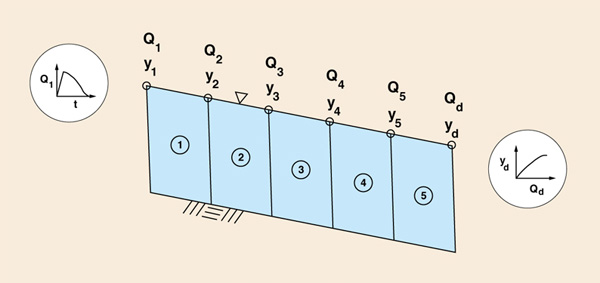
Stream Channel Routing
Stream channel routing uses mathematical relations to calculate outflow from a stream channel once inflow, lateral contributions, and channel characteristics are known.
Stream channel routing usually implies open channel flow conditions, although there are exceptions, such as storm sewer flow, for which mixed open channel-closed conduit flow conditions may prevail.
In this chapter, stream channel routing refers to unsteady flow calculations in streams and rivers.
Channel reach refers to a specific length of stream channel possessing certain translation and storage properties.
The hydrograph at the upstream end of the reach is the inflow hydrograph; the hydrograph at the downstream end is the outflow hydrograph.
Lateral contributions consist of point tributary inflows and/or distributed inflows; e.g., interflow and groundwater flow.
The terms stream channel routing and flood routing are often used interchangeably.
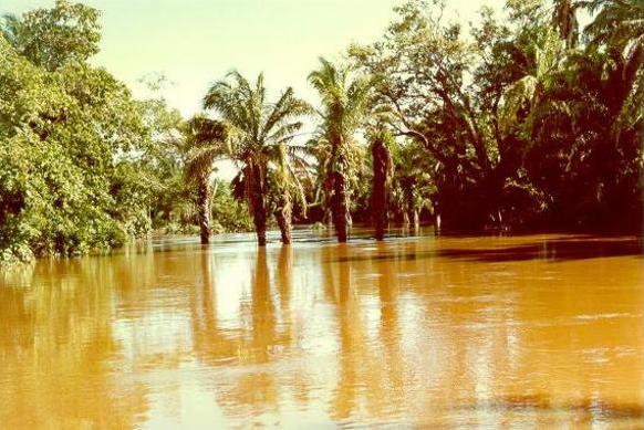
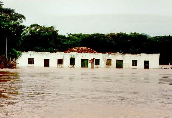
This is attributed to the fact that most stream channel routing applications are in flood flow analysis, flood control design, or flood forecasting (Fig. 9-1).
Figure 9-1 Flood stage in a tropical river. |
Two general approaches to stream channel routing are recognized: (1) hydrologic and (2) hydraulic.
As in the case of reservoir routing (Chapter 8), hydrologic stream channel routing is based on the storage concept.
Conversely, hydraulic channel routing is based on the principles of mass and momentum conservation.
Hydraulic routing techniques are of three types: (1) kinematic wave, (2) diffusion wave, and (3) dynamic wave.
The dynamic wave is the most complete model of unsteady open channel flow.
Kinematic and diffusion waves are convenient and practical approximations to the dynamic wave.
An alternate approach to hydrologic and hydraulic routing has emerged in recent years.
This approach is similar in nature to the hydrologic routing methods yet contains sufficient physical information to compare favorably with the more complex hydraulic routing techniques.
This hybrid approach is the basis of the Muskingum-Cunge method of flood routing.
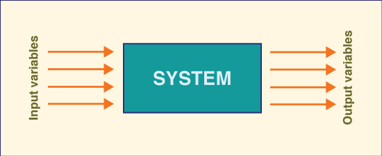
At the outset of the study of stream channel routing, it is necessary to introduce a few basic modeling concepts.
A typical hydrologic model consists of: (1) input, (2) system, and (3) output (Fig. 9-2).
In surface water hydrology, the system is usually a catchment, a reservoir, or a stream channel.
In the case of a catchment, the input is a storm hyetograph.
For reservoirs and stream channels, the input is an inflow hydrograph.
For all three cases, catchments, reservoirs, and channels, the output is an outflow hydrograph.
Figure 9-2 Input, system, and output in a typical hydrologic model. |
In general, modeling problems are classified into three types: (1) prediction, (2) calibration, and (3) inversion.
In the prediction problem, input and system are known and described by properties or parameters, and the task is to calculate the output based on the knowledge of system and input.
For instance, with known inflow hydrograph, lateral contributions, and channel reach parameters, the outflow hydrograph from a stream channel can be computed using routing techniques (Example 9-1).
In the calibration problem, input and output are known, and the objective is to determine the properties or parameters describing the system.
In the case of a stream channel, with known upstream inflow, lateral contributions, and outflow hydrograph, the routing parameters are calculated by a calibration procedure (Example 9-2).
The inversion problem is the third type of modeling problem.
In this case, system and output are known, and the task is to calculate the inflow or inflows. This is accomplished by reversing the routing process in a technique known as inverse channel routing.
For instance, with known upstream inflow, outflow, and channel reach parameters, the lateral contributions can be calculated by inverse routing.
The prediction problem is the more common type of modeling application; however, a calibration is usually required in advance of the prediction.
Model verification is the process of testing the model with actual data to establish its predictive accuracy.
To calibrate and verify a model, it is usually necessary to assemble two different data sets.
The first set is used in model calibration and the second set is used in model verification.
A close agreement between calculated and measured data is an indication that the model has been verified.
A detailed discussion of these subjects is given in Chapter 13.
Muskingum Method
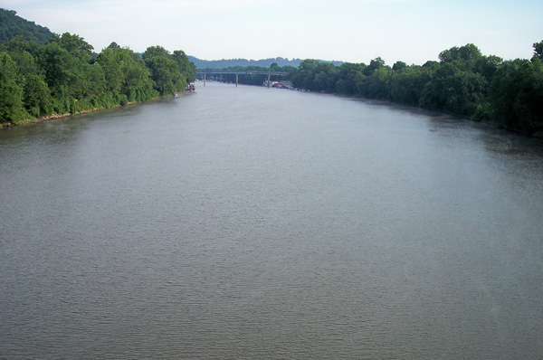
The Muskingum method of flood routing was developed in the 1930s in connection with the design of flood protection schemes in the Muskingum River Basin, Ohio (Fig. 9-3) [11].
It is the most widely used method of hydrologic stream channel routing, with numerous applications in the United States and throughout the world.
Figure 9-3 The Muskingum river near Marietta, Ohio. |
The Muskingum method is based on the differential equation of storage, Eq. 8-4, reproduced here:
|
dS I - O = _____ dt | (8-4) |
In an ideal channel, storage is a function of inflow and outflow.
This is in constrast with an ideal reservoir, in which storage is solely a function of outflow (see Eqs. 8-5 to 8-7).
In the Muskingum method, storage is a linear function of inflow and outflow:
| S = K [ X I + ( 1 - X ) O ] | (9-1) |
in which S = storage volume; I = inflow; O = outflow; K = a time constant or storage coefficient; and X = a dimensionless weighting factor.
With inflow and outflow in cubic meters per second, and K in hours, storage volume is in (cubic meters per second)-hour.
Alternatively, K could be expressed in seconds, in which case storage volume is in cubic meters.
Equation 9-1 was developed in 1938 and has been widely used since then [11].
It is esentially a generalization of the linear reservoir concept (Eq. 8-7).
In fact, for X = 0, Eq. 9-1 reduces to Eq. 8-7.
In other words, linear reservoir routing is a special case of Muskingum channel routing for which
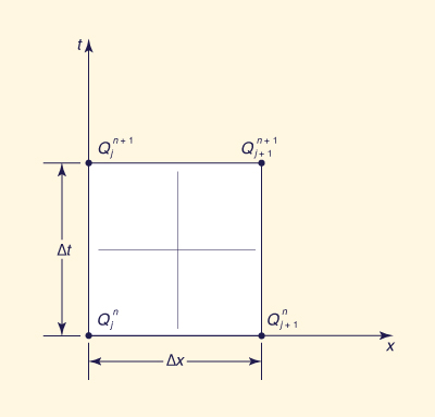
To derive the Muskingum routing equation, Eq. 8-4 is discretized on the x-t plane (Fig. 8-2), to yield Eq. 8-13, repeated here:
|
I1 + I2 O1 + O2 S2 - S1 __________ - ___________ = ___________ 2 2 Δt | (8-13) |
Equation 9-1 is expressed at time levels 1 and 2:
| S1 = K [ X I1 + ( 1 - X ) O1 ] | (9-2) |
| S2 = K [ X I2 + ( 1 - X ) O2 ] | (9-3) |
Substituting Eqs. 9-2 to 9-3 into Eq. 8-13 and solving for O2 yields Eq. 8-15, repeated here:
| O2 = C0 I2 + C1 I1 + C2 I1 | (8-15) |
in which C0, C1 and C2 are routing coefficients defined in terms of Δt, K, and X as follows:
|
( Δt / K ) - 2X C0 = _______________________ 2(1 - X) + ( Δt / K ) | (9-4) |
|
( Δt / K ) + 2X C1 = _______________________ 2(1 - X) + ( Δt / K ) | (9-5) |
|
2(1 - X) - ( Δt / K ) C2 = _______________________ 2(1 - X) + ( Δt / K ) | (9-6) |
Since C0 + C1 + C2 = 1, the routing coefficients may be interpreted as weighting coefficients.
For
Given an inflow hydrograph, an initial flow condition, a chosen time interval Δt, and routing parameters X and K, the routing coefficients can be calculated with Eqs. 9-4 to 9-6, and the outflow hydrograph with Eq. 8-15.
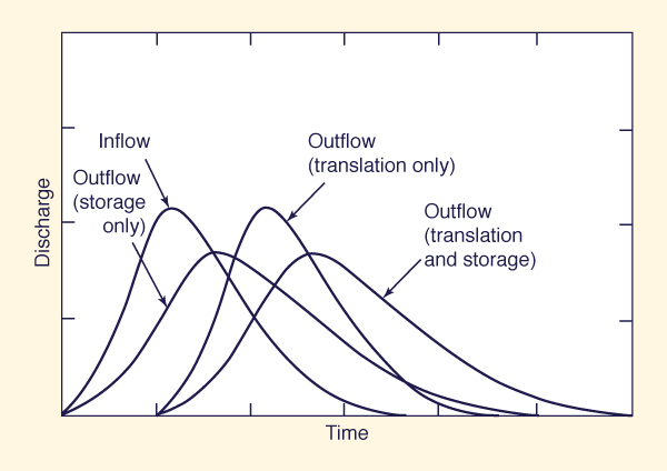
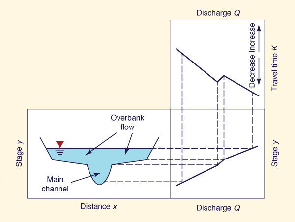
The routing parameters K and K are related to flow and channel characteristics, K being interpreted as the travel time of the flood wave from upstream end to downstream end of the channel reach.
Therefore, K accounts for the translation (or concentration) portion of the routing (Fig. 9-3).
The parameter X accounts for the storage portion of the routing.
For a given flood event, there is a value of X for which the storage in the calculated outflow hydrograph matches that of the measured outflow hydrograph.
The effect of storage is to reduce the peak flow and spread the hydrograph in time (Fig. 9-4).
Therefore, it is often used interchangeably with the terms diffusion and peak attenuation.
Figure 9-4 Translation and storage processes in stream channel routing. |
The routing parameter K is a function of channel reach length and flood wave speed; conversely, the parameter X is a function of the flow and channel characteristics that cause runoff diffusion.
In the Muskingum method, X is interpreted as a weighting factor and restricted in the range 0.0 ≤ X ≤ 0.5.
Values of X greater than 0.5 produce hydrograph amplification (i.e., negative diffusion), which does not correspond with reality (under the Froude numbers applicable to flood flows).
With K = Δt and X = 0.5, flow conditions are such that the outflow hydrograph retains the same shape as the inflow hydrograph, but it is translated downstream a time equal to K.
For X = 0, Muskingum routing reduces to linear reservoir routing (Section 8.2).
In the Muskingum method, the parameters K and X are determined by calibration using streamflow records.
Simultaneous inflow-outflow discharge measurements for a given channel reach are coupled with a trial-and-error procedure, leading to the determination of K and X (see Example 9-2).
The procedure is time-consuming and lacks predictive capability. Values of K and X determined in this way are valid only for the given reach and flood event used in the calibration.
Extrapolation to other reaches or to other flood events (of different magnitude) within the same reach is usually unwarranted.
When sufficient data are available, a calibration can be performed for several flood events, each of different magnitude, to cover a wide range of flood levels.
In this way, the variation of K and X as a function of flood level can be ascertained.
In practice, K is more sensitive to flood level than X.
A sketch of the variation of K with stage and discharge is shown in Fig. 9-5.
Figure 9-5 Sketch of travel time as a function of discharge and stage. |
Example 9-1.
An inflow hydrograph to a channel reach is shown in Col. 2 of Table 9-1.
Assume baseflow is 352 m3/s.
Using the Muskingum method, route this hydrograph through a channel reach with K = 2 d and X = 0.1 to calculate an outflow hydrograph.
First, it is necessary to select a time interval Δt.
In this case, it is convenient to choose Δt = 1 d.
As with reservoir routing, the ratio of time-to-peak to time interval (tp/Δt) should be greater than or equal to 5.
In addition, the chosen time interval should be such that the routing coefficients remain positive.
With Δt = 1 d, K = 2 d, and X = 0.1, the routing coefficients (Eqs. 9-4 to 9-6) are: C0 = 0.1304; C1 = 0.3044; and C2 = 0.5652.
It is verified that C0 + C1 + C2 = 1.
The routing calculations are shown in Table 9-1.
Column 1 shows the time in days.
Column 2 shows the inflow hydrograph ordinates in cubic meters per second.
Columns 3-5 show the partial flows.
Following Eq. 8-15, Cols. 3-5 are summed to obtain Col. 6, the outflow hydrograph ordinates in cubic meters per second.
To explain the procedure briefly, the outflow at the start (day 0) is assumed to be equal to the inflow at the start: 352 m3/s. The inflow at day 1 multiplied by C0 is entered in Col. 3, day 1: 76.6 m3/s.
The inflow at day 0 multiplied by C1 is entered in Col. 4, day
1: 107.1 m3/s.
The outflow at day 0 multiplied by C2 is entered in Col. 5, day 1: 199 m3/s.
Columns 3-5 of day 1 are summed to obtain Col. 6 of day 1: 76.6 + 107.1 + 199.0 = 382.7 m3/s.
The calculations proceed in a recursive manner until all outflows in Col. 6 have been obtained.
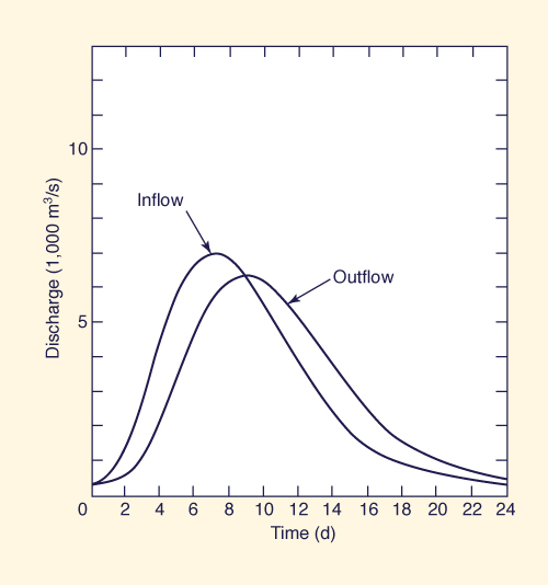
Inflow and outflow hydrographs are plotted in Fig. 9-6.
The outflow peak is 6352.6 m3/s, which shows that the inflow peak, 6951 m3/s, has attenuated to about 91 % of its initial value.
The peak outflow occurs at day 9, 2 d after the peak inflow, which occurs at day 7.
The time elapsed between the occurrence of peak inflow and peak outflow is generally equal to K, the travel time.
ONLINE CALCULATION.
Using ONLINE ROUTING04, the answer
is essentially the same as that of Col. 6, Table 9-1.
| ||||||||||||||||||||||||||||||||||||||||||||||||||||||||||||||||||||||||||||||||||||||||||||||||||||||||||||||||||||||||||||||||||||||||||||||||||||||||||||||||||||||||||||||||||||||
Figure 9-6 Stream channel routing by Muskingum method: Example 9-1. |
Unlike reservoir routing, stream channel-routing calculations exhibit a definite (time) lag between inflow and outflow.
Furthermore, in the general case (X ≠ 0), maximum outflow does not occur at the time when inflow and outflow coincide.
Example 9-1 has illustrated the predictive stage of the Muskingum method, in which the routing parameters are known in advance of the routing.
If the parameters are not known, it is first necessary to perform a calibration.
The trial-and-error procedure to calibrate the routing parameters is illustrated by Example 9-2.
Example 9-2.
Use the outflow hydrograph calculated in the previous example together with the given
inflow hydrograph to calibrate the Muskingum method, that is, to find the routing parameters K and X.
The procedure is summarized in Table 9-2.
Column 1 shows the time in days.
Column 2 shows the inflow hydrograph in cubic meters per second.
Column 3 shows the outflow hydrograph in cubic meters per second.
Column 4 shows the channel storage in (cubic meters per second)-days.
Channel storage at the start is assumed to be 0, and this value is entered in Col. 4, day 0.
Channel storage is calculated by solving Eq. 8-13 for S2:
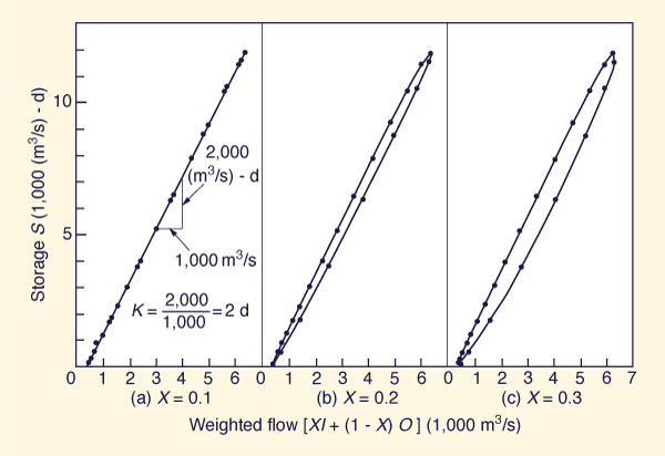
Several values of X are tried, within the range 0.0 to 0.5, for example, 0.1, 0.2 and 0.3.
For each trial value of X, the weighted flows [ XI + ( 1 - X ) O ] are calculated, as shown in Cols. 5-7.
Each of the weighted flows is plotted against channel storage (Col. 4), as shown in Fig. 9-7.
The value of X for which the storage versus weighted flow data plots closest to a line is taken as the correct value of X.
In this case, Fig. 9-7 (a): X = 0.1 is chosen.
Following Eq. 9-1, the value of K is obtained from Fig. 9-7 (a) by calculating the slope of the storage vs weighted outflow curve.
In this case, the value of K = [2000 (m3/s)-d]/(1000 m3/s) = 2 d.
Thus, it is shown that K = 2 days and X = 0.1 are the Muskingum routing parameters for the given inflow and outflow hydrographs.
| |||||||||||||||||||||||||||||||||||||||||||||||||||||||||||||||||||||||||||||||||||||||||||||||||||||||||||||||||||||||||||||||||||||||||||||||||||||||||||||||||||||||||||||||||||||||||||||||||||||||||||||||||
Figure 9-7 Calibration of Muskingum routing parameters: Example 9-2. |
The estimation of routing parameters is crucial to the application of the Muskingum method.
The parameters are not constant, tending to vary with flow rate.
If the routing parameters can be related to flow and channel characteristics, the need for trial-and-error calibration would be eliminated.
Parameter K could be related to reach length and flood wave velocity, whereas X could be related to the diffusivity characteristics of flow and channel.
These propositions are the basis of the Muskingum-Cunge method (Section 9.4).
9.2 KINEMATIC WAVES
|
|
Three types of unsteady open-channel flow waves are commonly used in engineering
hydrology:
Kinematic waves are the simplest type of wave and dynamic waves are the most complex; diffusion waves lie somewhere in between kinematic and dynamic waves.
Kinematic waves are discussed in this section and diffusion waves are discussed in Section 9.3.
An introduction to dynamic waves is given in Section 9.5.
Kinematic Wave Equation
The derivation of the kinematic wave equation is based on the principle of mass conservation within a control volume.
This principle states that the difference between outflow and inflow within one time interval is balanced by a corresponding change in volume. In terms of finite intervals (i.e., finite differences) it is:
| ( Q2 - Q1 ) Δt + ( A2 - A1 ) Δx = 0 | (9-8) |
in which Q = flow; A = flow area; Δt = time interval; and Δx = space interval.
In differential form,
|
∂Q ∂A ____ + ____ = 0 ∂x ∂t | (9-9) |
which is the equation of conservation of mass, or equation of continuity.
The equation of conservation of momentum (Eq. 4-22) contains local inertia, convective inertia, pressure gradient (due to flow depth gradient), friction (friction slope), gravity (bed slope), and a momentum source term (Section 4.2).
In deriving the kinematic wave equation, a statement of uniform flow is used in lieu of conservation of momentum.
Since uniform flow is strictly a balance of friction and gravity, it follows that local and convective inertia, pressure gradient, and momentum source terms are excluded from the formulation of kinematic waves.
In other words, a kinematic wave is a simplified wave that does not include these terms or processes.
As shown later in this section, this simplification imposes limits to the applicability of kinematic waves.
Uniform flow in open channels is described by the Manning or Chezy formulas (Section 2.4). The Manning equation is:
|
1 Q = ___ A R 2/3 Sf 1/2 n | (9-10) |
in which R is the hydraulic radius in meters, Sf is the friction slope in meters per meter, and n is the Manning friction coefficient.
A pictorial on n is given by Barnes (1967).
The Chezy equation is:
|
Q = C A R 1/2 Sf 1/2 | (9-11) |
in which C = Chezy coefficient.
Notice that in unsteady flow, friction slope is used in Eqs. 9-10 and 9-11 in lieu of channel slope.
The hydraulic radius is R = A/P, in which P is the wetted perimeter.
Substituting this into Eq. 9-10, leads to:
|
1 Sf 1/2 Q = ___ _________ A5/3 n P 2/3 | (9-12) |
Assume for the sake of simplicity that n, Sf, and P are constant.
This may be the case of a wide channel in which P can be assumed to be essentially independent of A.
Equation 9-12 can then be written as:
| Q = α Aβ | (9-13) |
in which α and β are parameters of the discharge-area rating (see rating curve, Section 2.4), defined as follows:
|
1 Sf 1/2 α = ___ _________ n P 2/3 | (9-14) |
|
5 β = ___ 3 | (9-15) |
In Eq. 9-13, differentiating Q with respect to A leads to:
|
dQ Q _____ = β ____ = β V dA A | (9-16) |
in which V is the mean flow velocity.
Multiplying Eqs. 9-9 and 9-16 and applying the chain rule, the kinematic wave equation is obtained:
|
∂Q dQ ∂Q _____ + (_____) ______ = 0 ∂t dA ∂x | (9-17) |
or, alternatively
|
∂Q ∂Q _____ + (β V) ______ = 0 ∂t ∂x | (9-18) |
Equation 9-17 (or 9-18) describes the movement of waves which are kinematic in nature.
These are referred to as kinematic waves, i.e., waves for which inertia and pressure (flow depth) gradient have been neglected [10].
Equation 9-17 is a first-order partial differential equation.
Therefore, kinematic waves travel with wave celerity dQ/dA (or βV) and do not attenuate.
Wave attenuation can only be described by a second-order partial differential equation.
The absence of wave attenuation can be further explained by resorting to a mathematical argument.
Since dQ/dA is the celerity of the unsteady (i.e. , wavelike) Q, it can be replaced by dx/dt.
Therefore, in Eq. 9-17:
|
∂Q dx ∂Q _____ + (_____) ______ = 0 ∂t dt ∂x | (9-19) |
which is equal to the total derivative dQ/dt.
Since the right side of Eq. 9-19 is zero, it follows that Q remains constant in time for waves traveling with celerity dQ/dA.
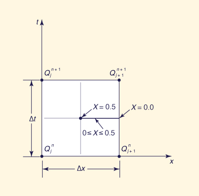
Discretization of Kinematic Wave Equation
Equation 9-18 (or 9-17) is a nonlinear first-order partial differential equation describing the change of discharge Q in time and space.
It is nonlinear because the wave celerity βV (or dQ/dA) varies with discharge.
The nonlinearity, however, is usually mild, and therefore, Eq. 9-18 can also be solved in a linear mode by considering the wave celerity to be constant.
The solution of Eq. 9-18 can be obtained by analytical or numerical means.
The simplest kinematic wave solution is a linear numerical solution.
For this purpose, it is necessary to select a numerical scheme with which to discretize Eq. 9-18 on the x-t plane (Fig. 9-8).
A review of basic concepts of numerical analysis is necessary before discussing numerical schemes.
Figure 9-8 Space-time discretization of kinematic wave equation. |
Order of Accuracy of Numerical Schemes
The order of accuracy of a numerical scheme measures the ability of the scheme to reproduce (i.e., recreate) the terms of the differential equation.
In general, the higher the order of accuracy of a scheme, the better it is able to reproduce the terms of the differential equation.
Forward and backward finite differences have first-order accuracy, i.e., discretization errors of first order.
Central differences have second-order accuracy, with discretization errors of second order.
When solving Eq. 9-18 by numerical methods, first-order schemes create numerical diffusion and numerical dispersion, while second-order schemes create only numerical dispersion.
A third-order scheme creates neither numerical diffusion nor dispersion.
Numerical diffusion and/or dispersion are caused by the finite grid size and are not necessarily related to the physical problem.
Second-order-accurate Numerical Scheme
The discretization of Eq. 9-18 following a linear second-order-accurate scheme, i.e., using central differences in space and time, leads to (Fig. 9-8):
|
M N ______ + βV ______ = 0 Δt Δx | (9-20) |
|
Q j+1n+1 + Q j n+1 Q j+1n + Q j n M = ___________________ - _________________ 2 2 | (9-20a) |
|
Q j+1n + Q j+1 n+1 Q j n + Q j n+1 N = ___________________ - _________________ 2 2 | (9-20b) |
in which βV has been held constant (linear mode), leading to:
| Q j+1 n+1 = C0 Q j n+1 + C1 Q j n + C2 Q j+1 n | (9-21) |
in which
|
C - 1 C0 = _______ 1 + C | (9-22) |
| C1 = 1 | (9-23) |
|
1 - C C2 = _______ 1 + C | (9-24) |
and C is the Courant number, defined as follows:
|
Δt C = βV _____ Δx | (9-25) |
Note that Courant number is the ratio of physical wave celerity βV to grid celerity Δx /Δt.
The Courant number is a fundamental concept in the numerical solution of hyperbolic partial differential equations.
Example 9-3.
Use Eq. 9-21 with the routing coefficients of Eqs. 9-22 to 9-24 (linear kinematic wave numerical solution using central differences in space and time) to route the following triangular flood wave.
Consider the following three cases: (1) V = 1.2 m/s and Δx = 7200 m; (2) V = 1.2 m/s and Δx = 4800 m; and (3) V = 0.8 mls and Δx = 4800 m. Use β = 5/3, and Δt = 1 h.
Using Eq. 9-25: C = 1.
Using Eqs. 9-22 to 9-24: C0 = 0; C1 = 1; C2 = 0.
The routing by Eq. 9-21 shown in Table 9-3 depicts the pure translation of the hydrograph a time equal to Δt.
In other words, for βV = Δx/Δt (i.e., C = 1), the central difference scheme is of third order, and the numerical solution is exactly equal to the analytical solution.
Using Eq. 9-25: C = 1.5.
Using Eqs. 9-22 to 9-24: C0 = 0.2; C1 = 1.0; C2 = -0.2.
The routing by Eq. 9-21 shown in Table 9-4 depicts the translation of the hydrograph a time approximately equal to Δt, but it also shows a small amount of numerical dispersion because βV
is not equal to Δx/Δt.
The dispersion, including the notorious negative
outflows at the trailing end of the hydrograph, are caused by errors associated with the scheme's second-order accuracy.
Using Eq. 9-25, C = 1.
Therefore, the solution is the same as in the first case, exhibiting pure hydrograph translation.
| |||||||||||||||||||||||||||||||||||||||||||||||||||||||||||||||||||||||||||||||||||||||||||||||||||||||||||||||||||||||||||||||||||||||||||||||||||||||||||||||||||||||||||||||||||||||||||||||||||||||||||||||||||||||||||||||||
The three cases of Example 9-3 illustrate the properties of kinematic waves.
The second-order-accurate scheme has no numerical diffusion.
In addition, for Courant number C = 1, i.e., the wave celerity βV equal to the grid celerity Δx/Δt, the scheme has no numerical dispersion, with the hydrograph being translated downstream without change in shape.
In other words, the numerical solution by Eqs. 9-21 to 9-25 is exact only for Courant number C = 1.
For other values of C, the numerical solution exhibits perceptible amounts of numerical dispersion.
First-order-accurate Numerical Scheme
The numerical solution of Eq. 9-18 can also be attempted using a first-order-accurate scheme, i.e., one featuring forward or backward finite differences.
The discretization of Eq. 9-18 in a linear mode, using backward differences in both space and time yields (Fig. 9-8):
|
Q j+1n+1 - Q j+1 n Q j+1n+1 - Q j n+1 ____________________ + βV ___________________ = 0 Δt Δx | (9-26) |
from which
| Q j+1n+1 = C0 Q j n+1 + C2 Q j+1n | (9-27) |
in which
|
C C0 = _________ 1 + C | (9-28) |
|
1 C2 = _________ 1 + C | (9-29) |
and C = Courant number, defined by Eq. 9-25.
Example 9-4.
Use Eq. 9-27 with the coefficients calculated by Eq. 9-28 and 9-29 to route the same inflow hydrograph as in the previous example.
Use V = 1.2 m/s; Δx = 7200 m; β = 5/3; and Δt = 1 h.
Using Eq. 9-25, C = 1.
Therefore, C0 = 0.5, and C2 = 0.5.
The routing using Eq. 9-27 is shown in Table 9-5.
It is observed that off-centering the derivatives by using backward differences has caused a significant amount of numerical diffusion, with peak outflow of 120.93 m3/s as compared to peak inflow of 150 m3/s.
The conclusion is that different schemes for solving Eq. 9-18 lead to different answers, depending on the time and space intervals, Courant number, order of accuracy of the scheme, and associated numerical diffusion and/or dispersion.
| ||||||||||||||||||||||||||||||||||||||||||||||||||||||||||||||||||||||||||||||||||||||||||||||||||||||||||||||||||||||
Convex Method
The convex method of stream channel routing belongs to the family of linear kinematic wave methods.
Through the 1970s, it was part of the SCS TR-20 model for hydrologic simulation (Chapter 13).
The routing equation for the convex method is obtained by discretizing Eq. 9-18 in a linear mode using a forward-in-time, backward-in-space finite difference scheme, to yield (Fig. 9-8):
|
Q j+1n+1 - Q j+1n Q j+1n - Q j n __________________ + βV ________________ = 0 Δt Δx | (9-30) |
from which
| Q j+1n+1 = C1 Q j n + C2 Q j+1n | (9-31) |
in which
| C1 = C | (9-32) |
| C2 = 1 - C | (9-33) |
and C = Courant number (Eq. 9-25), restricted to C ≤ 1 for numerical stability reasons.
In the convex method, C is regarded as an empirical routing coefficient.
Example 9-5 illustrates the application of the convex method.
The convex method is relatively simple, but the solution is dependent on the routing parameter C.
The latter could be interpreted as a Courant number and related to kinematic wave celerity and grid size, as in Eq. 9-25.
However, for values of C other than 1, the amount of diffusion introduced in the numerical problem is unrelated to the true diffusion, if any, of the physical problem.
Therefore, the convex method, as well as all kinematic wave methods featuring uncontrolled amounts of numerical diffusion, are regarded as a somewhat crude approach to stream channel routing.
Example 9-5.
Use Eq. 9-31 (the convex method) to route the same inflow hydrograph as in Example 9-3.
Assume C = 2/3.
The routing coefficients are C1 = C = 2/3; and C2 = 1 - C = 1/3.
The routing is shown in Table 9-6.
The convex method leads to a significant amount of diffusion, with peak outflow of 135.06 m3/s as compared to peak inflow of 150 m3/s.
The calculated diffusion amount is a function of C, with practical values of C being restricted in the range 0.5 to 0.9.
For C = 1, the hydrograph is translated with no diffusion or dispersion, as in the first and third parts of Example 9-3.
Values of C > 1 render the calculation unstable (large negative values of discharge) and are,
therefore, not recommended.
It should be noted that the instability of the convex method for C > 1 has a parallel in the instability of the Muskingum method for X > 0.5.
| ||||||||||||||||||||||||||||||||||||||||||||||||||||||||||||||||||||||||||||||||||||||||||||||||||||||||||||||||
Kinematic Wave Celerity
The kinematic wave celerity is dQ/dA, or βV.
A value of β = 5/3 was derived for the case of a hydraulically wide channel governed by Manning friction.
The kinematic wave celerity is also known as the Kleitz-Seddon, or Seddon, law [8, 19].
In 1900, Seddon [19] published a paper in which he studied the nature of unsteady flow movement in rivers and concluded that the celerity of long disturbances was equal to:
|
1 dQ c = ____ _____ T dy | (9-34) |
in which dQ/dy = slope of the discharge-stage rating (Q versus y), and T = stage, or water surface elevation.
The quantity c is the kinematic wave celerity.
Since dA = T dy, the kinematic wave celerity is equal to dQ/dA (see Eq. 9-17) [10].
From Eq. 9-34 it is concluded that the kinematic wave celerity is a function of the slope of the discharge-stage rating.
This slope is likely to vary with stage; therefore, the kinematic wave celerity is not constant but varies with stage and flow level.
If c = βV is a function of Q, then Eq. 9-18 is a nonlinear equation requiring an iterative solution.
Nonlinear kinematic wave solutions account for the variation of kinematic wave celerity with stage and flow level.
The simpler linear solutions, as in Examples 9-3 and 9-4, assume a constant value of kinematic wave celerity βV.
Notice that there is a striking similarity between the linear kinematic wave solutions and the Muskingum method.
This subject is further examined in Section 9.4.
Theoretical β values other than 5/3 can be obtained for other friction formulations and cross-sectional shapes.
For turbulent flow governed by Manning friction, β has an upper limit of 5/3, and it is usually greater than 1.
For laminar flow in wide channels, β = 3; for mixed or transitional flow-between laminar and turbulent Manning, it is in the range 5/3 < β < 3.
For flow in a hydraulically wide channel described by the Chezy formula, β = 3/2 (Section 4.2).
The calculation of β as a function of frictional type and cross-sectional shape is illustrated by the following example.
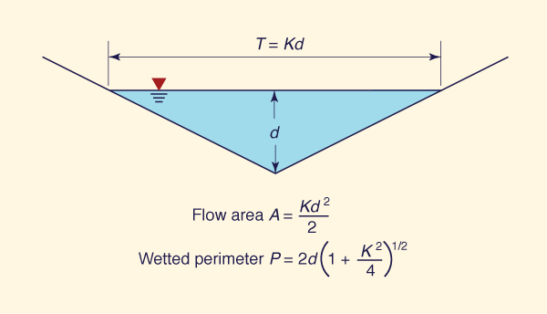
Example 9-6.
Calculate the value of β
for a triangular channel with Manning friction.
Equation 9-10 is the Manning equation.
Substituting R = A/P leads to Eq. 9-12.
Since P is a function of A, Eq. 9-12 can be written as follows:
in which K1 is a constant containing n and Sf .
The latter have been assumed to be independent of either A or P.
For the triangular-shaped channel of Fig. 9-9, the top width is proportional to the flow depth, say
Figure 9-9 Properties of a triangular channel cross section.
and the wetted perimeter is:
Eliminating d from Eqs. 9-36 and 9-37:
from which
in which K2 is a constant containing K.
Substituting Eq. 9-39 into Eq. 9-35 leads to:
in which K3 is a constant containing
K1 and K2.
From Eq. 9-40:
and the value of β for a triangular channel with Manning friction is β = 4/3.
|
Kinematic Waves with Lateral Inflow
Practical applications of stream channel routing often require the specification of lateral inflows.
The latter could be either concentrated, as in the case of tributary inflow at a point along the channel reach, or distributed along the channel, as with groundwater exfiltration (for effluent streams) or infiltration (for influent streams).
As with Eq. 9-9, a mass balance leads to:
|
∂Q ∂A ____ + ____ = qL ∂x ∂t | (9-42) |
which, unlike Eq. 9-9, includes the source term qL, the lateral flow per unit channel length.
For Q given in cubic meters per second and x in meters, qL is given in cubic meters per second per meter [L2 T -1].
Multiplying Eq. 9-42 by ∂Q / ∂A (or βV), as with Eq. 9-17 (or Eq. 9-18), leads to:
|
∂Q ∂Q _____ + (β V) ______ = (β V) qL ∂t ∂x | (9-43) |
which is the kinematic wave equation with lateral inflow (or outflow).
For qL positive, there is lateral inflow (e.g., tributary flow); for qL negative, there is lateral outflow (e.g., channel transmission losses).
Applicability of Kinematic Waves
The kinematic wave celerity is a fundamental streamflow property.
Flood waves which approximate kinematic waves travel with the kinematic wave celerity (c = βV) and are subject to very little or no attenuation.
In practice, flood waves are kinematic if they are of long duration (Fig. 9-10) or travel on a channel of steep slope.
Criteria for the applicability of kinematic waves to overland flow [20] (Section 4.2) and stream channel flow [14] have been developed.
The stream channel criterion states that in order for a wave to be kinematic, it should satisfy the following dimensionless inequality:
|
tr So Vo __________ ≥ M do | (9-44) |
in which tr is the time-of-rise of the inflow hydrograph, So is the bottom slope, Vo is the average velocity, and do is the average flow depth.
For 95% accuracy in one period of translation, a value of
Figure 9-10 Flood stage in a large tropical river. |
Example 9-7.
Use the kinematic wave criterion (Eq. 9-44) to determine whether a flood wave with the following characteristics is a kinematic wave: time-of-rise tr = 12 h;
bottom slope So = 0.001;
average velocity
For the given channel and flow characteristics, the left side of Eq. 9-44 is equal to 43.2, which is less than 85.
For values greater than 85, the wave would be kinematic-therefore, subject to negligible diffusion.
Since the value is 43.2, this wave is not kinematic and is likely to experience a significant amount of diffusion.
If this wave is routed as a kinematic wave with zero diffusion and dispersion, as in Example 9-3 (Part 1), the peak outflow would be much larger than in reality.
If this wave is routed as a kinematic wave with diffusion or dispersion, as in Examples 9-3 (Part 2) and 9-4, it is likely that the amount of numerical diffusion and/or dispersion would be different from the actual amount of physical diffusion.
It should be noted that had the bottom slope been So = 0.01, the left side of Eq. 9-44 would be 432, satisfying the kinematic wave criterion.
Therefore, it is concluded that the steeper the channel slope, the more kinematic the flow is.
ONLINE CALCULATION.
Using ONLINE KINEMATIC WAVE APPLICABILITY, the answer
is |
9.3 DIFFUSION WAVES
|
|
In Section 9.1, the Muskingum method was used to calculate unsteady flows in a hydrologic sense.
In Section 9.2, the principle of mass conservation was coupled with a uniform flow formula to derive the kinematic wave equation.
Solutions to this equation have been widely used in hydrologic practice, particularly for overland flow and other routing applications involving steep slopes or slow-rising hydrographs.
The Muskingum method and linear kinematic wave solutions show striking similarities.
Both methods have the same type of routing equation.
The Muskingum method, however, can calculate hydrograph diffusion, whereas the kinematic wave can do so only by the introduction of numerical diffusion.
The latter is dependent on the grid size and type of numerical scheme.
Kinematic wave theory can be enhanced by allowing a small amount of physical diffusion in its formulation [10].
In this way, an improved type of kinematic wave can be formulated, a kinematic-with-diffusion wave, for short, a diffusion wave.
A definite advantage of the diffusion wave is that it includes the diffusion which is present in most natural unsteady open channel flows.
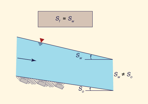
Diffusion Wave Equation
In Section 9.2, the kinematic wave equation was derived by using a statement of steady uniform flow (i.e., friction slope is equal to bottom slope) in lieu of momentum conservation.
In deriving the diffusion wave, a statement of steady nonuniform flow (i.e., friction slope is equal to water surface slope) is used instead (Fig. 9-11).
This leads to:
|
1 dy Q = ___ A R 2/3 ( So - ____ ) 1/2 n dx | (9-45) |
in which the term [So - (dy/dx)] is the water surface slope.
The difference between kinematic and diffusion waves is in the term dy/dx.
From a physical standpoint, the term dy/dx accounts for the natural diffusion processes present in unsteady open channel flow phenomena.
Figure 9-11 Diffusion wave assumption. |
To derive the diffusion wave equation, Eq. 9-45 is expressed in a slightly different form:
|
dy m Q 2 = So - ____ dx | (9-46) |
in which m is the reciprocal of the square of the channel conveyance K, defined as:
|
1 K = ___ A R 2/3 n | (9-47) |
With dA = T dy, in which T = top width, Eq. 9-46 changes to:
|
1 dA _____ ______ + m Q 2 - So = 0 T dx | (9-48) |
Equations 9-9 and 9-48 constitute a set of two partial differential equations describing diffusion waves.
These equations can be combined into one equation with Q as dependent variable.
However, it is first necessary to linearize the equations around reference flow values.
For simplicity, a constant top width is assumed (i.e., a wide channel assumption).
The linearization of Eqs. 9-9 and 9-48 is accomplished by small perturbation theory [4].
This procedure, while heuristic, has seemed to work well in a number of applications.
The variables Q, A, and m can be expressed in terms of the sum of a reference value (with subscript o) and a small perturbation to the reference value (with superscript '): Q = Qo + Q' ; A = Ao + A' ; m = mo + m'.
Substituting these into Eqs. 9-9 and 9-48, neglecting squared perturbations, and subtracting the reference flow leads to:
|
∂Q' ∂A' ____ + ____ = 0 ∂x ∂t | (9-49) |
and
|
1 ∂A' _____ ______ + Qo2 m' + 2 mo Qo Q' = 0 T ∂x | (9-50) |
Differentiating Eq. 9-49 with respect to x and Eq. 9-50 with respect to t gives:
|
∂2Q' ∂2A' ______ + _______ = 0 ∂x2 ∂x ∂t | (9-51) |
|
1 ∂2A' ∂m' ∂Q' _____ _________ + Qo2 _____ + 2 mo Qo ______ = 0 T ∂x ∂t ∂t ∂t | (9-52) |
Using the chain rule and Eq. 9-49 yields:
|
∂m' ∂m' ∂A' ∂m' ∂Q' _____ = _______ _______ = - _______ _______ ∂t ∂A' ∂t ∂A' ∂x | (9-53) |
Combining Eq. 9-52 with Eq. 9-53:
|
1 ∂2A' ∂m' ∂Q' ∂Q' _____ ________ - Qo2 ______ ______ + 2 mo Qo ______ = 0 T ∂x ∂t ∂A' ∂x ∂t | (9-54) |
Combining Eqs. 9-51 and 9-54 and rearranging terms, yields:
|
∂Q' Qo ∂m' ∂Q' 1 ∂Q'2 ______ - _______ ______ ______ = _____________ _______ ∂t 2 mo ∂A' ∂x 2 T mo Qo ∂x2 | (9-55) |
Since by definition: mQ 2 = Sf, it follows that
|
∂Q' ∂Q Qo _____ = _______ = - _______ ∂m' ∂m 2 mo | (9-56) |
and also
|
So mo Qo = ______ Qo | (9-57) |
Substituting Eqs. 9-56 and 9-57 into Eq. 9-55, using the chain rule, and dropping the superscripts for simplicity, the following equation is obtained:
|
∂Q ∂Q ∂Q Qo ∂2Q ______ + ( ______ ) ______ = ( __________ ) _______ ∂t ∂A ∂x 2 T So ∂x2 | (9-58) |
The left side of Eq. 9-58 is recognized as the kinematic wave equation, with ∂Q/∂A as the kinematic wave celerity.
The right side is a second-order (partial differential) term that accounts for the physical diffusion effect.
The coefficient of the second-order term has the units of diffusivity
The hydraulic diffusivity is a characteristic of the flow and channel, defined as:
|
Qo qo νh = _________ = _______ 2 T So 2 So | (9-59) |
in which qo = Qo/T is the reference flow per unit of channel width.
From Eq. 9-59, it is concluded that the hydraulic diffusivity is small for steep bottom slopes (e.g., those of small mountain streams), and large for mild bottom slopes (e.g., tidal rivers).
Equation 9-58 describes the movement of flood waves in a better way than Eq. 9-17 or 9-18.
It falls short from describing the full momentum effects, but it does physically account for peak flow attenuation.
Equation 9-58 is a second-order parabolic partial differential equation.
It can be solved analytically, leading to Hayami's diffusion analogy solution for flood waves [7], or numerically with the aid of a numerical scheme for parabolic equations such as the Crank-Nicolson scheme [3].
An alternate approach is to match the hydraulic diffusivity with the numerical diffusion coefficient of the Muskingum scheme.
This approach is the basis of the Muskingum-Cunge method [4, 12] (Section 9.4).
Applicability of Diffusion Waves
Most flood waves have a small amount of physical diffusion; therefore, they are better approximated by the diffusion wave rather than by the kinematic wave.
For this reason, diffusion waves apply to a much wider range of practical problems than kinematic waves.
Where the diffusion wave fails, only the dynamic wave can properly describe the translation and diffusion of flood waves.
The dynamic wave, however, is very strongly diffusive, especially for flows well in the subcritical regime [14].
In practice, most flood flows are only mildly diffusive, and therefore, are subject to modeling with the diffusion wave.
To determine if a wave is a diffusion wave, it should satisfy the following dimensionless inequality [14]:
|
g tr So ( ____ )1/2 ≥ N do | (9-60) |
in which tr is the time-of-rise of the inflow hydrograph, So is the bottom slope, do is the average flow depth, and g is the gravitational acceleration.
The greater the left side of this inequality, the more likely it is that the wave is a diffusion wave.
In practice, a value of N = 15 is recommended for general use.
Example 9-8.
Use the criterion of Eq. 9-60 to determine whether the flood wave of Example 9-7 can be considered a diffusion wave.
For tr = 12 h, So = 0.001, and do = 2 m, the left side of Eq. 9-60 is 95.7, which is greater than 15.
In the previous example, this wave was shown not to satisfy the kinematic wave criterion.
This example shows, however, that this wave is a diffusion wave. Had Eq. 9-60 not been satisfied, the flood wave would have been properly a dynamic wave, subject only to dynamic wave routing.
Dynamic wave routing takes into account the complete momentum quation, including the inertia terms (local and convective) that were neglected in the formulation of kinematic and diffusion waves. Section 9.5 contains a brief introduction to dynamic waves.
ONLINE CALCULATION.
Using ONLINE KINEMATIC WAVE APPLICABILITY, the answer
is |
9.4 MUSKINGUM-CUNGE METHOD
|
|
The Muskingum method can calculate runoff diffusion, ostensibly by varying the parameter X.
A numerical solution of the linear kinematic wave equation using a third-order accurate scheme (C = 1) leads to pure flood hydrograph translation (see Example 9-3, Part 1).
Other numerical solutions to the linear kinematic wave equation invariably produce a certain amount of numerical diffusion and/or dispersion (See Example 9-3, Part 2).
The Muskingum and linear kinematic wave routing equations are strikingly similar.
Furthermore, unlike the kinematic wave equation, the diffusion wave equation does have the capability to describe physical diffusion.
From these propositions, Cunge [4] concluded that the Muskingum method is a linear kinematic wave solution and that the flood wave attenuation shown by the calculation is due to the numerical diffusion of the scheme itself.
To prove this assertion, the kinematic wave equation (Eq. 9-18) is discretized on the x-t plane (Fig. 9-12) in a way that parallels the Muskingum method, centering the spatial derivative and off-centering the temporal derivative by means of a weighting factor X:
|
X (Q j n+1 - Q j n ) + (1 - X) (Q j+1n+1 - Q j+1 n ) ________________________________________________ + Δt |
|
(Q j+1 n - Q j n ) + (Q j+1n+1 - Q
j n+1 ) c _______________________________________ = 0 2 Δx | (9-61) |
in which c = βV is the kinematic wave celerity.
Figure 9-12 Space-time discretization of kinematic wave equation paralleling Muskingum method. |
Solving Eq. 9-61 for the unknown discharge leads to the following routing equation:
| Q j+1 n+1 = C0 Q j n+1 + C1 Q j n + C2 Q j+1 n | (9-62) |
The routing coefficients are:
|
c ( Δt / Δx ) - 2X C0 = ________________________ 2(1 - X) + c ( Δt / Δx ) | (9-63) |
|
c ( Δt / Δx ) + 2X C1 = ________________________ 2(1 - X) + c ( Δt / Δx ) | (9-64) |
|
2(1 - X) - c ( Δt / Δx ) C2 = ________________________ 2(1 - X) + c ( Δt / Δx ) | (9-65) |
By defining the travel time
|
Δx K = ______ c | (9-66) |
it is seen that the two sets of Eqs. 9-63 to 9-65 and Eqs. 9-4 to 9-6 are the same.
Equation 9-66 confirms that K is in fact the flood wave travel time, i.e., the time it takes a given discharge to travel the reach length Δx with the kinematic wave celerity c.
In a linear mode, c is constant and equal to a reference value; in a nonlinear mode, it varies with discharge.
It can be seen that for X = 0.5, Eqs. 9-63 to 9-65 reduce to the routing coefficients of the linear second-order-accurate kinematic wave solution, Eqs. 9-22 to 9-24.
For X = 0.5 and C = 1 (C =
For X = 0.5 and C ≠ 1, it is second-order accurate, exhibiting only numerical dispersion (recall that in the context of convection-diffusion, numerical dispersion is the error of the second-order scheme).
For X< 0.5 and C ≠ 1, it is first-order accurate, exhibiting both numerical diffusion and dispersion.
For X < 0.5 and C = 1, it is first: order accurate, exhibiting only numerical diffusion (effectively, the numerical dispersion vanishes for C = 1).
These relations are summarized in Table 9-7.
| ||||||||||||||||||||||||||||||
In practice, the numerical diffusion can be used to simulate the physical diffusion of the actual flood wave.
By expanding the discrete function Q (jΔx, n Δt) in Taylor series about grid point (jΔx, n Δt), the numerical diffusion coefficient of the Muskingum scheme is derived (see Appendix B):
|
1 νn = c Δx ( ____ - X ) 2 | (9-67) |
in which νn is the numerical diffusion coefficient of the Muskingum scheme.
This equation reveals the following:
For X = 0.5 there is no numerical diffusion, although there is numerical dispersion for C ≠ 1;
For X > 0.5, the numerical diffusion coefficient is negative, i.e., numerical amplification, which explains the behavior of the Muskingum method for this range of X values;
For Δx = 0, the numerical diffusion coefficient is zero, clearly the trivial case.
A predictive equation for X can be obtained by matching the hydraulic diffusivity νh (Eq. 9-59) with the numerical diffusion coefficient of the Muskingum scheme νn (Eq. 9-67). This leads to the following expression for X:
|
1 qo X = ___ ( 1 - __________ ) 2 So c Δx | (9-68) |
With X calculated by Eq. 9-68, the Muskingum method is referred to as Muskingum-Cunge method [12].
Using Eq. 9-68, the routing parameter X can be calculated as a function of the following numerical and physical properties:
Reach length Δx,
Reference discharge per unit width qo,
Kinematic wave celerity c, and
Bottom slope So.
It should be noted that Eq. 9-68 was derived by matching physical and numerical diffusion (i.e., second-order processes), and does not account for dispersion (a third-order process).
Therefore, in order to simulate wave diffusion properly with the Muskingum-Cunge method, it is necessary to optimize numerical diffusion (with Eq. 9-68) while minimizing numerical dispersion by keeping the value of C as close to 1 as practicable.
A unique feature of the Muskingum-Cunge method is the grid independence of the calculated outflow hydrograph, which sets it apart from other linear kinematic wave solutions featuring uncontrolled numerical diffusion and dispersion (e.g., the convex method).
If numerical dispersion is minimized, the calculated outflow at the downstream end of a channel reach will be essentially the same, regardless of how many subreaches are used in the computation.
This is because X is a function of Δx,
and the routing coefficients C0, C1,
and
An improved version of the Muskingum-Cunge method is due to Ponce and Yevjevich [15].
The C value is the Courant number, i.e. , the ratio of wave celerity c to grid celerity Δx/ Δt:
|
Δt C = c ______ Δx | (9-69) |
The grid diffusivity is defined as the numerical diffusivity for the case of X = 0.
From Eq. 9-67, the grid diffusivity is:
|
Δx νg = c _____ 2 | (9-70) |
The cell Reynolds number [18] is defined as the ratio of hydraulic diffusivity (Eq. 9-59) to grid diffusivity (Eq. 9-70).
This leads to:
|
qo D = __________ So c Δx | (9-71) |
in which D = cell Reynolds number. Therefore:
|
1 X = ___ ( 1 - D ) 2 | (9-72) |
Equations 9-71 and 9-72 imply that for very small values of Δx, D may be greater than 1, leading to negative values of X. In fact, for the characteristic reach length
|
qo Δxc = ________ So c | (9-73) |
the cell Reynolds number is D = 1, and X = 0.
Therefore, in the Muskingum-Cunge method, reach lengths shorter than the characteristic reach length result in negative values of X.
This should be contrasted with the classical Muskingum method (Section 9.1), in which X is restricted in the range 0.0 ≤ X ≤ 0.5.
In the classical Muskingum, X is interpreted as a weighting factor.
As shown by Eqs. 9-71 and 9-72, nonnegative values of X are associated with long reaches, typical of the manual computation used in the development and early application of the Muskingum method.
In the Muskingum-Cunge method, however, X is interpreted in a moment-matching sense [2] or diffusion-matching factor.
Therefore, negative values of X are entirely possible.
This feature allows the use of shorter reaches than would otherwise be possible if X were restricted to nonnegative values.
The substitution of Eqs. 9-69 and 9-72 into Eqs. 9-63 to 9-65 leads to routing coefficients expressed in terms of Courant and cell Reynolds numbers:
|
-1 + C + D C0 = ______________ 1 + C + D | (9-74) |
|
1 + C - D C1 = ______________ 1 + C + D | (9-75) |
|
1 - C + D C2 = ______________ 1 + C + D | (9-76) |
The calculation of routing parameters C and D, Eqs. 9-69 and 9-71, can be performed in several ways.
The wave celerity can be calculated with either Eq. 9-16 or Eq. 9-34.
With Eq. 9-16, c = βV; with Eq. 9-34, c = (1/T) dQ/dy.
Theoretically, these two equations are the same.
For practical applications, if a stage-discharge rating and cross-sectional geometry are available (i.e., stage-discharge-top width tables), Eq. 9-34 is preferred over Eq. 9-16 because it accounts directly for cross-sectional shape.
In the absence of a stage-discharge rating and cross-sectional data, Eq. 9-16 can be used to estimate flood wave celerity.
With the aid of Eqs. 9-69 and 9-71, the routing parameters may be based on flow characteristics.
The calculations can proceed in a linear or nonlinear mode.
In the linear mode, the routing parameters are based on reference flow values and kept constant throughout the computation in time.
The choice of reference flow has a bearing on the calculated results [2, 15], although the overall effect is likely to be small.
For practical applications, either an average or peak flow value can be used as reference flow.
The peak flow value has the advantage that it can be readily ascertained, although a better approximation may be obtained by using an average value [15].
The linear mode of computation is referred to as the constant-parameter Muskingum-Cunge method to distinguish it from the variable-parameter Muskingum-Cunge method, in which the routing parameters are allowed to vary with the flow.
The constant parameter method resembles the Muskingum method, with the difference that the routing parameters are based on measurable flow and channel characteristics instead of historical streamflow data.
Example 9-9.
Use the constant-parameter Muskingum-Cunge method to route a flood wave with the following flood and channel characteristics: peak flow Qp = 1000 m3/s; baseflow Qb, = 0 m3/s; channel bottom slope So = 0.000868; flow area at peak discharge Ap = 400 m2; top width at peak discharge Tp = 100 m; rating exponent β = 1.6; reach length Δx = 14.4 km; time interval Δt = 1 h.
The mean velocity (based on the peak discharge) is V = Qp/Ap = 2.5 m/s.
The wave celerity is c = βV =
ONLINE CALCULATION.
Using ONLINE ROUTING05, the answer
is essentially the same as that of Col. 6, Table 9-8.
| |||||||||||||||||||||||||||||||||||||||||||||||||||||||||||||||||||||||||||||||||||||||||||||||||||||||||||||||||||||||||||||||||||||||
Resolution Requirements
When using the Muskingum-Cunge method, care should be taken to ensure that the values of Δx and Δt are sufficiently small to approximate closely the actual shape of the hydrograph.
For smoothly rising hydrographs, a minimum value of tp /Δt = 5 is recommended.
This requirement usually results in the hydrograph time base being resolved into at least 15 to 25 discrete points, considered adequate for Muskingum routing.
Unlike temporal resolution, there is no definite criteria for spatial resolution.
A criterion borne out by experience is based on the fact that Courant and cell Reynolds numbers are inversely related to reach length Δx.
Therefore, to keep Δx sufficiently small, Courant and cell Reynolds numbers should be kept sufficiently large.
This leads to the practical criterion [16]:
| C + D ≥ 1 | (9-77) |
which can be written as follows: -1 + C + D ≥ 0.
This confirms the necessity of avoiding negative values of C0 in Muskingum-Cunge routing (see Eq. 9-74).
Experience has shown that negative values of either C1 or C2 do not adversely affect the method's overall accuracy [16].
Notwithstanding Eq. 9-77, the Muskingum-Cunge method works best when the numerical dispersion is minimized, that is, when C ≅ 1.
Values of C substantially less than 1 are likely to cause the notorious dips, or negative outflows, in portions of the calculated hydrograph.
This computational anomaly is attributed to excessive numerical dispersion and should be avoided.
Nonlinear Muskingum-Cunge Method
The kinematic wave equation, Eq. 9-18, is nonlinear because the kinematic wave celerity varies with discharge.
The nonlinearity is mild, among other things because the wave celerity variation is usually restricted within a narrow range.
However, in certain cases it may be necessary to account for this nonlinearity.
This can be done in two ways: (1) during the discretization, by allowing the wave celerity to vary, resulting in a nonlinear numerical scheme to be solved by iterative means; and (2) after the discretization, by varying the routing parameters, as in the variable-parameter Muskingum-Cunge method [15].
The latter approach is particularly useful if the overall nonlinear effect is small, which is often the case.
In the variable parameter method, the routing parameters are allowed to vary with the flow.
The values of C and D are based on local qo and c values instead of peak flow or other reference value as in the constant-parameter method.
To vary the routing parameters, the most expedient way is to obtain an average value of qo and c for each computational cell.
This can be achieved with a direct three-point average of the values at the known grid points (see Fig. 9-11), or by an iterative four-point average, which includes the unknown grid point.
To improve the convergence of the iterative four-point procedure, the three-point average can be used as the first guess of the iteration.
Once qo and c have been determined for each computational cell, the Courant and cell Reynolds numbers are calculated by Eqs. 9-69 and 9-71.
The value of bottom slope So remains unchanged within each computational cell.
The variable parameter Muskingum-Cunge method represents a small yet sometimes perceptible improvement over the constant parameter method.
The differences are likely to be more marked for very long reaches and/or wide variations in flow levels.
Flood hydrographs calculated with variable parameters show a certain amount of distortion, either wave steepening in the case of flows contained inbank or wave attenuation (flattening) in the case of typical overbank flows.
This is a physical manifestation of the nonlinear effect, i.e., different flow levels traveling with different celerities.
On the other hand, flood hydrographs calculated using constant parameters do not show wave distortion.
Assessment of Muskingum-Cunge Method
The Muskingum-Cunge method is a physically based alternative to the Muskingum method.
Unlike the Muskingum method where the parameters are calibrated using streamflow data, in the Muskingum-Cunge method the parameters are calculated based on flow and channel characteristics.
This makes possible channel routing without the need for time-consuming and cumbersome parameter calibration.
More importantly, it makes possible extensive channel routing in ungaged streams with a reasonable expectation of accuracy.
With the variable-parameter feature, nonlinear properties of flood waves (which could otherwise only be obtained by more elaborate numerical procedures) can be described within the context of the Muskingum formulation.
Like the Muskingum method, the Muskingum-Cunge method is limited to diffusion waves.
Furthermore, the Muskingum-Cunge method is based on a single-valued rating and does not take into account strong flow non-uniformity or unsteady flows exhibiting substantial loops in discharge-stage rating (i.e., dynamic waves).
Thus, the Muskingum-Cunge method is suited for channel routing in natural streams without significant backwater effects and for unsteady flows that classify under the diffusion wave criterion (Eq. 9-60).
An important difference between the Muskingum and Muskingum-Cunge methods should be noted.
The Muskingum method is based on the storage concept (Chapter 4) and, therefore, it is lumped, with the parameters K and X being reach averages.
The Muskingum-Cunge method, however, is distributed in nature, with the parameters C and D being based on values evaluated at channel cross sections.
Therefore, for the Muskingum-Cunge method to improve on the Muskingum method, it is necessary that the routing parameters evaluated at channel cross sections be representative of the channel reach under consideration.
Historically, the Muskingum method has been calibrated using streamflow data.
On the contrary, the Muskingum-Cunge method relies on physical characteristics such as rating curves, cross-sectional data and channel slope.
The different data requirements reflect the different theoretical bases of the methods, i.e., lumped storage concept in the Muskingum method, and distributed kinematic/diffusion wave theory in the Muskingum-Cunge method.
9.5 INTRODUCTION TO DYNAMIC WAVES
|
|
In Section 9.2, kinematic waves were formulated by simplifying the momentum conservation principle to a statement of steady uniform flow.
In Section 9.3, diffusion waves were formulated by simplifying the momentum principle to a statement of steady nonuniform flow.
These two waves, in particular the diffusion wave, have been extensively used in stream channel routing applications.
The Muskingum and Muskingum-Cunge methods are examples of calculations using the concept of diffusion wave.
A third type of open channel flow wave, the dynamic wave, is formulated by taking into account the complete momentum principle, including its inertial components.
As such, the dynamic wave contains more physical information than either kinematic or diffusion waves.
Dynamic wave solutions, however, are more complicated than either kinematic or diffusion wave solutions.
In a dynamic wave solution, the equations of mass and momentum conservation are solved by a numerical procedure, either the method of finite differences, the method of characteristics, or the finite element method.
In the method of finite differences, the partial differential equations are discretized following a chosen numerical scheme [9].
The method of characteristics is based on the conversion of the set of partial differential equations into a related set of ordinary differential equations, and the solution along a characteristic grid, i.e. a grid that follows characteristic directions (Fig. 4-16).
The method of finite elements solves a set of integral equations over a chosen grid of finite elements.
In the past four decades, the method of finite differences has come to be regarded as the most expedient way of obtaining a dynamic wave solution for practical applications [6, 9].
Among several numerical schemes that have been used in connection with the dynamic wave, the Preissmann scheme is perhaps the most popular.
This is a four-point scheme, centered in the temporal derivatives and slightly off-centered in the spatial derivatives.
The off-centering in the spatial derivatives introduces a small amount of numerical diffusion necessary to control the numerical stability of the nonlinear scheme.
This produces a workable yet sufficiently accurate scheme.
The stream channel is divided into several reaches for computational purposes (Fig. 9-12).
The application of the Preissmann scheme to the governing equations for the various reaches results in a matrix solution requiring a double sweep algorithm, i.e., one that accounts only for the nonzero entries of the coefficient matrix, which are located within a narrow band surrounding the main diagonal.
This technique leads to a considerable savings in storage and execution time.
With the appropriate upstream and downstream boundary conditions (Fig. 9-13), the solution of the set of hyperbolic equations marches in time until a specified number of time intervals is completed.
Figure 9-13 Reach subdivision for dynamic wave routing. |
In practice, a dynamic wave solution represents an order-of-magnitude increase in complexity and associated data requirements when compared to either kinematic or diffusion wave solutions.
Its use is recommended in situations where neither kinematic nor diffusion wave solutions are likely to represent adequately the physical phenomena.
In particular, dynamic wave solutions are applicable to flow over very flat slopes, flow into large reservoirs, strong backwater conditions and flow reversals.
In general, the dynamic wave is recommended for cases warranting a precise determination of the unsteady variation of river stages.
Relevance of Dynamic Waves to Engineering Hydrology
Dynamic wave solutions are often referred to as hydraulic river routing.
As such, they have the capability to calculate unsteady discharges and stages when presented with the appropriate geometric channel data and initial and boundary conditions.
Their relevance to engineering hydrology is examined here by comparing them to kinematic and diffusion wave solutions.
Kinematic waves calculate unsteady discharges; the corresponding stages are subsequently obtained from the appropriate rating curves.
Usually, equilibrium (steady, uniform) rating curves are used for this purpose.
Diffusion waves may or may not use equilibrium rating curves to calculate stages.
Some methods, e.g., Muskingum-Cunge, use equilibrium ratings, but more elaborate diffusion wave solutions may not.
Dynamic waves rely on the physics of the phenomena as built into the governing equations to generate their own unsteady rating.
A looped rating curve is produced at every cross section, as shown in Fig. 9-14.
For any given stage, the discharge is higher in the rising limb of the hydrograph and lower in the receding limb.
This loop is due to hydrodynamic reasons and should not be confused with other loops, which may be due to erosion, sedimentation, or changes in bed configuration (Chapter 15).
Figure 9-14 Sketch of the looped rating of dynamic waves. |
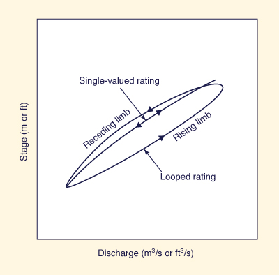
The width of the loop is a measure of the flow unsteadiness, with wider loops corresponding to highly unsteady flow, i.e., dynamic wave flow.
If the loop is narrow, it implies that the flow is mildly unsteady, perhaps a diffusion wave.
If the loop is practically nonexistent, the flow can be approximated as kinematic flow.
In fact, the basic assumption of kinematic flow is that momentum can be simulated as steady uniform flow, i.e., that the rating curve is single-valued.
The preceding observations lead to the conclusion that the relevance of dynamic waves in engineering hydrology is directly related to the flow unsteadiness and the associated loop in the rating curve.
For highly unsteady flows such as dam-break flood waves, it may well be the only way to properly account for the looped rating.
For other less unsteady flows, kinematic and diffusion waves are a viable alternative, provided their applicability can be clearly demonstrated (Eqs. 9-44 and 9-60).
Diffusion Wave Solution with Dynamic Component
A simplified approach to dynamic wave routing is that of the diffusion wave with dynamic component [2].
In this approach, the complete governing equations, including inertia terms, are linearized in a similar way as with diffusion waves.
This leads to a diffusion equation similar to Eq. 9-58, but with a modified hydraulic diffusivity.
The equation is [5]:
|
∂Q ∂Q ∂Q Qo ∂2Q ______ + ( ______ ) ______ = { ( ________ ) [ 1 - (β - 1)2 Fo2 ] } _______ ∂t ∂A ∂x 2 T So ∂x2 | (9-78) |
in which the hydraulic diffusivity (i.e., the coefficient of the second-order term) is also a function of the rating curve parameter β and the Froude number, defined as:
|
Vo Fo = ___________ (g do)1/2 | (9-79) |
with g = gravitational acceleration, and do = reference flow depth.
Equation 9-78 can be expressed in terms of the Vedernikov number [17]:
|
V = (β - 1) Fo
| (9-80) |
With Eq. 9-80, Eq. 9-78 reduces to:
|
∂Q ∂Q ∂Q Qo ∂2Q ______ + ( ______ ) ______ = [ ( ________ ) ( 1 - V 2 ) ] _______ ∂t ∂A ∂x 2 T So ∂x2 | (9-81) |
Equations 9-78 and 9-81 provide an enhanced predictive capability for the simulation of diffusion waves including a dynamic component.
For instance, for β = 1.5 (i.e., Chezy friction in wide channels) and Fo = 2, the Vedernikov number V = 1 (Eq. 9-80), and the hydraulic diffusivity vanishes, which is in agreement with physical reality [10, 13].
On the other hand, the hydraulic diffusivity of the diffusion wave (Eq. 9-58) is independent of the Vedernikov number.
Therefore, Eq. 9-81 is a better model than Eq. 9-58, especially for Froude numbers in the supercritical regime.
Most natural flows, however, are in the range well below critical, with Eq. 9-58 remaining a practical model of unsteady open channel flow phenomena [7].
QUESTIONS
|
|
What is routing? What types of waves are used in describing unsteady open channel flow processes?
What is model calibration? What is model verification?
In the Muskingum method, what does the parameter K represent? What does the parameter X represent?
How does channel routing differ from reservoir routing? What differences are to be noted in the routed hydrographs?
What is the kinematic wave celerity? What is the practical range of turbulent flow values of β, the rating constant used in the kinematic wave celerity?
What is the order of accuracy of a numerical scheme? What is the difference between numerical diffusion and numerical dispersion in connection with kinematic wave solutions?
What is a linear model in the context of kinematic wave routing? What is a nonlinear model?
Why are the results of convex routing dependent on the grid size?
What is a diffusion wave? How does it differ from a kinematic wave?
What is hydraulic diffusivity? Why is it important in flood routing?
What values of parameters X and C optimize numerical diffusion and minimize numerical dispersion in the Muskingum-Cunge method?
Why are negative values of X entirely possible in Muskingum-Cunge routing? Why are values of X in excess of 0.5 unfeasible?
What is the Courant number? What is the cell Reynolds number?
Describe the difference between linear and nonlinear solutions to channel routing problems.
What is a dynamic wave? How does it differ from the diffusion and kinematic waves?
How does the method of finite differences differ from the method of characteristics? What is a double sweep algorithm?
Discuss the influence of the loop in the rating in determining whether an open channel flow wave is dynamic in nature.
What is the Vederkinov number? How does it differ from the Froude number?
What is the effect of the inclusion of a dynamic component in diffusion wave modeling?
PROBLEMS
|
|
Given the following inflow hydrograph to a certain stream channel reach, calculate the outflow by the Muskingum method. Check your results with ONLINE ROUTING 04.
Time (h) 0 1 2 3 4 5 6 7 8 9 10 11 12 Flow (m3/s) 10 20 40 80 120 150 120 60 50 40 30 20 10 Assume K = 1 h, X = 0.2, and Δt = 1 h.
Given the following inflow hydrograph to a certain stream channel reach, calculate the outflow by the Muskingum method. Check your results with ONLINE ROUTING 04.
Time (h) 0 3 6 9 12 15 18 21 24 27 30 33 36 Flow (m3/s) 100 120 150 200 250 275 250 210 180 150 120 110 100 Assume K = 2.4 h, X = 0.1, and Δt = 3 h.
Given the following inflow and outflow hydrographs for a certain stream channel reach, calculate the Muskingum parameters K and X.
Time (h) 0 1 2 3 4 5 Inflow (ft3/s ) 2520 3870 4560 6795 8975 9320 Outflow (ft3/s ) 2520 2643 3598 4500 6367 8295 Time (h) 6 7 8 9 10 11 Inflow (ft3/s ) 7780 6520 5340 4105 3210 2520 Outflow (ft3/s ) 8900 7971 6808 5628 4439 3482 Time (h) 12 13 14 15 16 17 Inflow (ft3/s ) 2520 2520 2520 2520 2520 2520 Outflow (ft3/s ) 2782 2592 2540 2525 2521 2520 Develop a spreadsheet to solve the Muskingum method of stream channel routing, given the following data: (1) an inflow hydrograph of arbitrary shape, (2) baseflow, (3) storage constant K, (4) weighting factor X, and (5) time interval Δt. Test your spread sheet with Example 9-1 in the text. Check your results with ONLINE ROUTING 04.
Given the following inflow hydrograph, use the spread sheet developed in Problem 9-4 to calculate the outflow hydrograph by the Muskingum method.
Time (h) 0.00 0.25 0.50 0.75 1.0 1.25 1.50 1.75 2.0 2.25 2.50 2.75 Flow (m3/s) 0 1 2 4 8 10 8 6 4 2 1 0 Assume baseflow 0 m3/s, K = 0.4 h, X = 0.15, and Δt = 0.25 h. Check your results with ONLINE ROUTING 04.
Develop a spread sheet to estimate the parameters of the Muskingum method, given a matching set of inflow and outflow hydrographs for a certain channel reach. A suggested algorithm is to search for the value of X that minimizes the root mean square (RMS) of the differences between predicted and measured storage. For this purpose, several values of X (between the range 0.0 to 0.5) are tried. For each trial value, a regression line is fitted to the (measured) storage (calculated using Eq. 9-7) versus weighted flow data, with weighted flow in the abscissas and measured storage in the ordinates. The differences between measured storage and predicted storage, i.e., storage predicted by the regression, are calculated. The RMS is evaluated by the following formula:
1
RMS = [ ( ______ ) Σ (S - S' )2 ] 1/2
n - 1 n(9-82) in which S = measured storage, S' = predicted storage, and n = number of values. The X corresponding to the minimum RMS value is the estimated X. The Muskingum parameter K is the slope of the regression line corresponding to the chosen X value. Use Example 9-2 in the text to test your program.
Use the data of Problem 9-3 to test further the spread sheet developed in Problem 9-6.
Route the following flood wave using a linear forward-in-time/backward-in-space numerical scheme of the kinematic wave equation (similar to the convex method).
Time (min) 0 10 20 30 40 50 60 70 80 90 100 Flow (m3/s) 0 1 2 4 8 10 8 4 2 1 0 Derive the routing coefficients for a linear forward-in-space/ backward-in-time numerical scheme of the kinematic wave equation.
Use the routing coefficients derived in Problem 9-9 to route the inflow hydrograph of Problem 9-8. Assume a reach length Δx = 800 m.
Calculate the β value for a triangular channel with Chezy friction.
A large river of nearly constant width B = 900 m is seen to be rising at the rate of 10 cm/h. At the observation point, a stage measurement indicates that the current value of discharge is 2200 m3/s. What is a rough estimate of the discharge at a point 5 km upstream?
Solve Problem 9-12 if the tributary contribution between the two points is estimated to be constant and equal to 225 m3/s.
Determine if a flood wave with the following characteristics is a kinematic wave: time-of-rise tr = 6 h, bottom slope So = 0.015, average flow velocity Vo = 1.5 m/s, and average flow depth do = 3 m.
Determine if a flood wave with the following characteristics is a diffusion wave: time-of-rise
tr = 6 h, bottom slope So = 0.005, and average flow depthdo = 3 m. Program ONLINE_ROUTING_05 solves the Muskingum-Cunge method of flood routing, with routing parameters based on peak flow. Test this program using Example 9-9 in the text.
Run ONLINE_ROUTING_05 using the following data: peak discharge = 500 m3/s, time-to-peak = 5 h, time base = 15 h, channel bed slope = 0.0008, flow area corresponding to the peak discharge = 200 m2, channel top width corresponding to the peak discharge = 50 m, rating exponent β = 1.65, reach length = 15 km, time interval Δt = 1 h. Report peak outflow and time-to-peak.
Given the following inflow hydrograph to a stream channel reach, use ONLINE_ROUTING_05 to calculate the outflow hydrograph.
Time (h) 0 1 2 3 4 5 6 7 8 9 10 11 12 13 Flow (m3/s) 10 20 40 80 160 320 400 320 240 160 80 40 20 10 Assume channel bed slope = 0.001, flow area corresponding to the peak discharge = 800 m2, channel top width corresponding to the peak discharge = 35 m, rating exponent β = 1.6, reach length = 3 km, and time interval Δt = 1 h.
Given the following inflow hydrograph to a channel reach, calculate the outflow hydrographs for: (a) a reach length of 4 km, and (b) for a reach length of 5 km.
Time (h) 0 1 2 3 4 5 6 7 8 9 10 11 12 Flow (m3/s ) 5 8 12 20 28 33 29 22 19 13 8 6 5 Assume channel bed slope = 0.0015, flow area corresponding to the peak discharge = 42 m2, channel top width corresponding to the peak discharge = 18 m, and rating exponent β = 1.5.
Calculate the hydraulic diffusivity for the following flow conditions: channel bed slope = 0.002, mean flow depth 4 m, mean flow velocity 2 m/s, and rating exponent β = 1.6. Compare the two cases: (a) without inertia, and (b) with inertia.
REFERENCES
|
|
Abbott, M. A. (1975). "Method of Characteristics," in Unsteady Flow in Open Channels, Vol. 1, K. Mahmood and V. Yevjevich, editors, Fort Collins, Colorado: Water Resources Publications.
Agricultural Research Service, U.S. Department of Agriculture. (1973). "Linear Theory of Hydrologic Systems," Technical Bulletin No. 1468, (J. C. 1. Dooge, author), Washington, D.C.
Crandall. S. H. (1956). Engineering Analysis. Engineering Society Monographs. New York: McGraw-Hill.
Cunge. J. A. (1969). "On the Subject of a Flood Propagation Computation Method (Muskingum Method)," Journal of Hydraulic Research. Vol. 7, No.2, pp. 205-230.
Dooge, J. C. 1., W. B. Strupczewski, W.B. and J.J. Napiorkowski. (1982). "Hydrodynamic Derivation of Storage Parameters of the Muskingum Model," Journal of Hydrology. Vol. 54, pp. 371-387.
Fread, D. L. (1985). "Channel Routing," in Hydrological Forecasting. M. G. Anderson and T. P. Burt, editors. New York: John Wiley.
Hayami, S. (1951). "On the Propagation of Flood Waves," Bulletin of the Disaster Prevention Research Institute. Kyoto University, Kyoto, Japan, No.1, December.
Kleitz, M. (1877). "Note sur la Theorie du Mouvement non Permanent des Liquides et sur application a la Propagation del Crues des Rivieres, (Note on the Theory of Unsteady Flow of Liquids and on Application to Flood Propagation in Rivers)," Annales des Ponts et Chaussees, Ser. 5, Yol. 16, 2e semestre, pp. 133-196.
Liggett, J. A., and I. A. Cunge. (1975). "Numerical Methods of Solution of the Unsteady Flow Equations," in Unsteady Flow in Open Channels. Yol. 1, K. Mahmood and V. Yevjevich, editors. Fort Collins, Colorado: Water Resources Publications.
Lighthill, M. J., and G. B. Whitham. (1955). "On Kinematic Waves. I. Flood Movement in Long Rivers," Proceedings of the Royal Society of London. Vol. A229, May, pp. 281-316.
McCarthy, G. T. (1938). "The Unit Hydrograph and Flood Routing," unpublished manuscript, presented at a Conference of the North Atlantic Division, U.S. Army Corps of Engineers, June 24.
Natural Environment Research Council. (1975). Flood Studies Report. Vol. 3: Flood Routing. London. England.
Ponce, V. M., and D. B. Simons. (1977). "Shallow Wave Propagation in Open Channel Flow," Journal of the Hydraulics Division, ASCE, Vol. 103, No. HYI2, December, pp. 1461-1476.
Ponce, V. M., R. M. Li, and D. B. Simons. (1978). "Applicability of Kinematic and Diffusion Models." Journal of the Hydraulics Division, ASCE, Vol. 104, No. HY3, March, pp. 353-360.
Ponce, V. M., and V. Yevjevich. (1978). "Muskingum-Cunge Method with Variable Parameters," Journal of the Hydraulics Division, ASCE, Vol. 104, No. HY12, December, pp. 1663-1667.
Ponce, V. M., and F. D. Theurer. (1982). "Accuracy Criteria in Diffusion Routing," Journal of the Hydraulics Division, ASCE, Vol. 108, No. HY6, June, pp. 747-757.
Ponce, V. M. (1991). "New perspective on the Vedernikov number," Water Resources Research, Vol. 27, No. 7, July, pp. 1777-1779.
Roache. P. (1972). Computational Fluid Dynamics. Hermosa Publishers, New Mexico: Albuquerque.
Seddon, J. A. (1900). "River Hydraulics," Transactions, ASCE, Vol. 43, pp. 179-229.
Woolhiser. M. H., and J. A. Liggett. (1967). "Unsteady One-Dimensional Flow Over a Plane: The Rising Hydrograph." Water Resources Research. Vol. 3, No. 3, pp. 753-771.
SUGGESTED READINGS
Agricultural Research Service, U.S. Department of Agriculture. (1973). "Linear Theory of Hydrologic Systems." Technical Bulletin No. 1468, (J. C. I. Dooge, author), Washington, D.C.
Cunge, J. A. (1969). "On the Subject of a Flood Propagation Computation Method (Muskingum Method)." Journal of Hydraulic Research, Vol. 7. No.2. 1969, pp. 205-230.
Fread, D. L. (1985). "Channel Routing," in Hydrological Forecasting, M. G. Anderson and T. P. Burt, editors, New York: John Wiley.
Fread, D. L. (1993). "Flow Routing," Chapter 10 in Handbook of Hydrology, D. R. Maidment, editor, New York: McGraw-Hill.
Lighthill, M.J., and Whitham. G. B. (1955). "On Kinematic Waves. I. Flood Movement in Long Rivers," Proceedings of the Royal Society of London, Vol. A229, May, pp. 281-316.
Natural Environment Research Council. (1975). Flood Studies Report. Vol. 5: Flood Routing, London, England, 1975.
| http://engineeringhydrology.sdsu.edu |
|
150714 |