|
|
|
CHAPTER 6: FREQUENCY ANALYSIS |
|
"If the sediment load in a stream is reduced, equilibrium can be restored if the water discharge
or the bottom slope are reduced, or if the sediment diameter increases the proper amount." Emory W. Lane (1955) |
|
This chapter is divided into three sections. Section 6.1 contains a review of statistics and probability concepts useful in engineering hydrology. Section 6.2 describes techniques of flood frequency analysis. Section 6.3 discusses low-flow frequency and droughts. |
6.1 CONCEPTS OF STATISTICS
|
|
Introduction
The term frequency analysis refers to the techniques whose objective is to analyze the occurrence of hydrologic variables within a statistical framework, i.e., by using measured data and basing predictions on statistical laws.
These techniques are applicable to the study of statistical properties of either rainfall or runoff (flow) series.
In engineering hydrology, however, frequency analysis is commonly used to calculate flood discharges.
In principle, techniques of frequency analysis are applicable to gaged catchments with long periods of streamflow record.
In practice, these techniques are primarily used for large catchments, because these are more likely to be gaged and have longer record periods.
Frequency analysis is also applicable to midsize catchments, provided the record length is adequate.
For ungaged catchments (either midsize or large), frequency analysis can be used in a regional context to develop flow characteristics applicable to hydrologically homogeneous regions.
These techniques comprise what is referred to as regional analysis (Chapter 7).
The question to be answered by flow frequency analysis can be stated as follows: Given n years of daily streamflow records for stream S, what is the maximum (or minimum) flow Q that is likely to recur with a frequency of once in T years on the average?
Or, what is the maximum flow Q associated with a T-year return period?
Alternatively, frequency analysis seeks to answer the inverse question: What is the return period T associated with a maximum (or minimum) flow Q?
In more general terms, the preceding questions can be stated as follows:
Given n years of streamflow data for stream S and L years of design life of a certain structure, what is the probability P of a discharge Q being exceeded at least once during the design life L?
Alternatively, what is the discharge Q which has the probability P of being exceeded during the design life L?
Random Variables
Frequency analysis uses random variables and probability distributions.
A random variable follows a certain probability distribution.
A probability distribution is a function that expresses in mathematical terms the relative chance of occurrence of each of all possible outcomes of the random variable.
In statistical notation, P (X = x1) is the probability P that the random variable X takes on the outcome x1.
A shorter notation is P (x1).
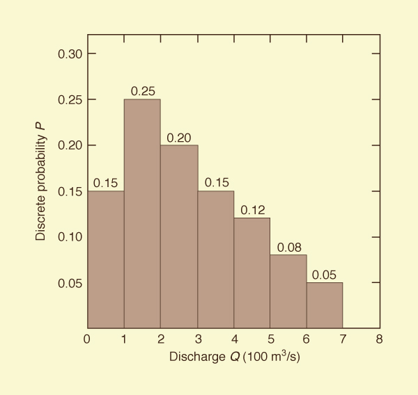
An example of random variable and probability distribution is shown in Fig. 6-1.
This is a discrete probability distribution because the possible outcomes have been arranged into groups (or classes).
The random variable is discharge Q; the possible outcomes are seven discharge classes, from 0-100 m3/s to 600-700 m3/s.
In Fig. 6-1, the probability that Q is in the class 100-200 m3/s is 0.25.
The sum of probabilities of all possible outcomes is equal to 1.
Figure 6-1 Discrete Probability Distribution. |
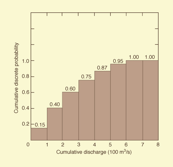
A cumulative discrete distribution, corresponding to the discrete probability distribution of Fig. 6-1, is shown in Fig. 6-2.
In this figure, the probability that Q is in a class less than or equal to the 100-200 m3/s class is 0.40.
The maximum value of probability of the cumulative distribution is 1.
Figure 6-2 Cumulative Discrete Probability Distribution. |
Properties of Statistical Distributions
The properties of statistical distributions are described by the following measures:
- Central tendency,
- Variability, and
- Skewness.
Statistical distributions are described in terms of moments.
The first moment describes central tendency, the second moment describes variability, and the third moment describes skewness.
Higher order moments are possible but are seldom used in practical applications.
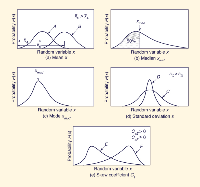
The first moment about the origin is the arithmetic mean, or mean.
It expresses the distance from the origin to the centroid of the distribution, as shown in Fig. 6-3 (a):
|
1 n x̄ = ____ Σ xi n i =1 | (6-1) |
in which x̄ is the mean, xi is the random variable, and n is the number of values.
The geometric mean is the nth root of the product of n terms:
| x̄ = (x1 x2 x3 . . . xn)1/n | (6-2) |
The logarithm of the geometric mean is the mean of the logarithms of the individual values.
The geometric mean is to the lognormal probability distribution what the arithmetic mean is to the normal probability distribution.
The median is the value of the variable that divides the probability distribution into two equal portions (or areas); see Fig. 6-3 (b).
For certain skewed distributions (i.e., one with third moment other than zero), the median is a better indication of central tendency than the mean.
Another measure of central tendency is the mode, defined as the value of the variable that occurs most frequently; see Fig. 6-3 (c).
Fig. 6-3 Properties of statistical distributions. |
Statistical moments can be defined about axes other than the origin.
The second moment about the mean is the variance, defined as
|
1 n s 2 = ________ Σ ( xi - x̄ ) 2 n - 1 i =1 | (6-3) |
in which s 2 is the variance.
The square root of the variance, s, is the standard deviation.
The variance coefficient (or coefficient of variation) is defined as
|
s Cv = ____ x̄ | (6-4) |
The standard deviation and variance coefficient are useful in comparing relative variability among distributions.
The larger the standard deviation and variance coefficient, the larger the spread of the distribution; see Fig. 6-3 (d).
The third moment about the mean is the skewness, defined as follows:
|
n n a = _______________ Σ ( xi - x̄ )3 (n - 1)(n - 2) i =1 | (6-5) |
in which a is the skewness. The skew coefficient is defined as
|
a Cs = ____ s3 | (6-6) |
For symmetrical distributions, the skewness is 0 and Cs = 0.
For right skewness (distributions with the long tail to the right), Cs > 0; for left skewness (long tail to the left), Cs < 0; see Fig. 6-3 (e).
Another measure of skewness is Pearson's skewness, defined as the ratio of the difference between mean and mode to the standard deviation.
Example 6-1.
Calculate the mean, standard deviation, and skew coefficient for the following flood series:
4580, 3490, 7260, 9350, 2510, 3720, 4070, 5400, 6220, 4350, and 5930 m3/ s.
The calculations are shown in Table 6-1.
Column 1 shows the year and Col. 2 shows the annual maximum flows.
The mean (Eq. 6-1) is calculated by summing up Col. 2 and dividing the sum by n = 11.
This results in x̄ = 5171 m3/s.
Column 3 shows the flow deviations from the mean, xi - x̄.
Column 4 shows the square of the flow deviations, ( xi - x̄ )2.
The variance (Eq. 6-3) is calculated by summing up Col. 4 and dividing the sum by (n - 1) = 10.
This results in: s 2 = 3,780,449 m6/ s2.
The square root of the variance is the standard deviation: s = 1944 m3/s.
The variance coefficient (Eq. 6-4) is Cv = 0.376.
Column 5 shows the cube of the flow deviations, ( xi - x̄ )3.
The skewness (Eq. 6-5) is calculated by summing up Col. 5 and multiplying
the sum by n / [(n - 1)(n - 2)] = 11/90.
This results in a = 6,717,359,675 m9/s3.
The skew coefficient (Eq. 6-6) is equal to the skewness divided by the cube of the standard deviation.
This results in Cs = 0.914.
| ||||||||||||||||||||||||||||||||||||||||||||||||||||||||||||||||||||||||||||
Continuous Probability Distributions
A continuous probability distribution is referred to as a probability density function (PDF).
A PDF is an equation relating probability, random variable, and parameters of the distribution.
Selected PDFs useful in engineering hydrology are described in this section.
Normal Distribution
The normal distribution is a symmetrical, bell-shaped PDF also known as the Gaussian distribution, or the natural law of errors.
It has two parameters: the mean μ, and the standard deviation σ, of the population.
In practical applications, the mean x̄ and the standard deviation s derived from sample data are substituted for μ and σ, respectively.
The PDF of the normal distribution is:
|
1 f (x) = __________ e - (x - μ)2 / (2σ2) σ (2π)1/2 | (6-7) |
in which x is the random variable and f (x) is the continuous probability.
By means of the transformation
|
x - μ z = ________ σ | (6-8) |
the normal distribution can be converted into a one-parameter distribution, as follows:
|
1 f (z) = ________ e-z 2/2 (2π)1/2 | (6-9) |
in which z is the standard unit, which is normally distributed with zero mean and unit standard deviation.
From Eq. 6-8:
| x = μ + z σ | (6-10) |
in which z, the standard unit, is the frequency factor of the normal distribution.
In general, the frequency factor of a statistical distribution is referred to as K.
A cumulative density function (CDF) can be derived by integrating the probability density function.
From Eq. 6-9, integration leads to
|
1 z F (z) = ________ ∫ e-u 2/2 du (2π)1/2 -∞ | (6-11) |
in which F(z) denotes cumulative probability and u is a dummy variable of integration.
The distribution is symmetrical with respect to the origin; therefore, only half of the distribution needs to be evaluated.
Table A-5 (Appendix A) shows values of F(z) versus z, in which F(z) is integrated from the origin to z.
Example 6-2.
The annual maximum flows of a certain stream have been found to be normally distributed, with mean 90 m3/s and standard deviation 30 m3/s.
Calcuiate the probability that a flow larger that 150 m3/s will occur.
To enter Table A-5, it is necessary to calculate the standard unit.
For a flow of 150 m3/s, the standard unit (Eq. 6-8) is: z = (150 - 90)/ 30 = 2.
This means that the flow of 150 m3/s is located two standard deviations to the right of the mean (had z been negative, the flow would have been located to the left of the mean).
In Table A-5, for z = 2, F(z) = 0.4772.
This value is the cumulative probability measured from z = 0 to z = 2, i.e., from the mean (90 m3/s) to the value being considered (150 m3/s).
Because the normal distribution is symmetrical with respect to the origin, the cumulative probability measured from z = - ∞ to z = 0, is 0.5.
Therefore, the cumulative probability measured from z = -∞ to z = 2, is F(z) = 0.5 + 0.4772 = 0.9772.
This is the probability that the flow is less than 150 m3/s.
To find the probability that the flow is larger than 150 m3/s,
the complementary cumulative probability is calculated: G(z)= 1 - F(z) = 0.0228.
Therefore, there is a (0.0228 × 100) = 2.28% chance that the annual maximum flow for the given stream will be larger than 150 m3/s.
|
Lognormal Distribution
For certain natural phenomena, values of random variables do not follow a normal distribution, but their logarithms do.
In this case, a suitable PDF can be obtained by substituting y for x in the equation for the normal distribution, Eq. 6-7, in which y = ln (x).
The parameters of the lognormal distribution are the mean and standard deviation of y : μy and σy.
Gamma Distribution
The gamma distribution is used in many applications of engineering hydrology.
The PDF of the gamma distribution is the following:
|
x γ - 1 e-x/β f (x) = _____________ β γ Γ(γ) | (6-12) |
for 0 < x < ∞, β > 0, and γ > 0.
The parameter γ is known as the shape parameter, since it most influences the peakedness of the distribution, while the parameter β is called the scale parameter, since most of its influence is on the spread of the distribution [4].
The mean of the gamma distribution is βγ, the variance is β2γ, and the skewness is 2/γ1/2.
The term Γ(γ) = (γ - 1)! , in which γ is a positive integer, is an important definite integral referred to as the gamma function, defined as follows:
|
∞ Γ(γ) = ∫ x γ - 1 e-x dx 0 | (6-13) |
Pearson Distributions
Pearson [24] has derived a series of probability functions to fit virtually any distribution.
These functions have been widely used in practical statistics to define the shape of many distribution curves.
The general PDF of the Pearson distributions is the following [6]:
|
x ∫ [( a + x ) / ( b0 + b1x + b2x2 )] dx -∞ f (x) = e | (6-14) |
in which a, b0 , b1, b2 are constants.
The criterion for determining the type of distribution is κ, defined as follows:
|
β1( β2 + 3)2 κ = ________________________________ 4 (4β2 - 3β1) (2β2 - 3β1 - 6) | (6-15) |
in which β1 = μ32/μ23 and β2 = μ4/μ22, with μ2, μ3, and μ4 being the second, third, and fourth moments about the mean.
With μ3 = 0 (i.e., zero skewness), β1 = 0, κ = 0, and the Pearson distribution reduces to the normal distribution.
The Pearson Type III distribution has been widely used in flood frequency analysis.
In the Pearson Type III distribution, κ = ∞, which implies that 2β2 = (3β1 + 6).
This is a three-parameter skewed distribution with the following PDF:
|
(x - xo)γ - 1 e - (x - xo) /β f (x) = _________________________ βγ Γ(γ) | (6-16) |
and parameters β, γ, and xo.
For xo = 0, the Pearson Type III distribution reduces to the gamma distribution (Eq. 6-12).
For γ = 1, the Pearson Type III distribution reduces to the exponential distribution, with the following PDF:
|
1 f (x) = (____) e- (x - xo) /β β | (6-17) |
The mean of the Pearson Type III distribution is: xo + βγ;
the variance is: β2γ; and
the skewness is:
Extreme Value Distributions
The extreme value distributions Types I, II, and III are based on the theory of extreme values.
Frechet (on Type II) in 1927 [8] and Fisher and Tippett (on Types I and III) in 1928 [8] independently studied the statistical distribution of extreme values.
Extreme value theory implies that if a random variable Q is the maximum in a sample of size n from some population of x values, then, provided n is sufficiently large, the distribution of Q is one of three asymptotic types (I, II, or III), depending on the distribution of x.
The extreme value distributions can be combined into one and expressed as a general extreme value (GEV) distribution [23].
The cumulative density function of the GEV distribution is:
| F ( x ) = e - [1 - k ( x - u ) / α]1/k | (6-18) |
in which k, u and α are parameters.
The parameter k defines the type of distribution, u is a location parameter, and α is a scale parameter.
For k = 0, the GEV distribution reduces to the extreme value Type I (EV1), or Gumbel distribution.
For k < 0, the GEV distribution is the extreme value Type II (EV2), or Frechet distribution.
For k > 0, the GEV distribution is the extreme value Type III (EV3), or Weibull distribution.
The GEV distribution is useful in applications where an extreme value distribution is being considered but its type is not known a priori.
Gumbel [13, 14, 15, 16] has fitted the extreme value Type I distribution to long records of river flows from many countries.
The cumulative density function (CDF) of the Gumbel distribution is the following double exponential function:
| F ( x ) = e -e -y | (6-19) |
in which y = (x - u)/α is the Gumbel (reduced) variate.
The mean ȳn and standard deviation σn of the Gumbel variate are functions of record length n.
Values of ȳn and σn as a function of n are given in Table A-8 (Appendix A).
When the record length approaches ∞, the mean ȳn approaches the value of the Euler constant (0.5772) [29], and the standard deviation σn approaches the value π /61/2.
The skew coefficient of the Gumbel distribution is 1.14.
The extreme value Type II distribution is also known as the log Gumbel.
Its cumulative density function is:
| F ( x ) = e -y 1/k | (6-20) |
for k < 0.
The extreme value Type III distribution has the same CDF as the Type II, but in this case k > 0.
As k approaches 0, the EV2 and EV3 distributions converge to the EV1 distribution.
6.2 FREQUENCY ANALYSIS
|
|
Flood frequency analysis refers to the application of frequency analysis to study the occurrence of floods.
Historically, many probability distributions have been used for this purpose.
The normal distribution was first used by Horton [19] in 1913, and shortly thereafter by Fuller [11].
Hazen [17] used the lognormal distribution to reduce skewness, whereas Foster [9] preferred to use the skewed Pearson distributions.
The logarithmic version of the Pearson Type III distribution, i.e., the log Pearson III, has been endorsed by the U.S. Interagency Advisory Committee on Water Data for general use in the United States [31].
The Gumbel distribution (extreme value Type I, or EVl) is also widely used in the United States and throughout the world.
The log Pearson III and Gumbel methods are described in this section.
Selection of Data Series
The complete record of streamflows at a given gaging station is called the complete duration series.
To perform a flood frequency analysis, it is necessary to select a flood series, i.e., a sample of flood events extracted from the complete duration series.
There are two types of flood series: (1) the partial duration series and (2) the extreme value series.
The partial duration (or peaks-over-a-threshold (POT) [23] series consists of floods whose magnitude is greater than a certain base value.
When the base value is such that the number of events in the series is equal to the number of years of record, the series is called an annual exceedance series.
In the extreme value series, every year of record contributes one value to the extreme value series, either the maximum value (as in the case of flood frequency analysis) or the minimum value (as in the case of low-flow frequency analysis).
The former is the annual maxima series; the latter is the annual minima series.
The annual exceedance series takes into account all extreme events above a certain base value, regardless of when they occurred.
However, the annual maxima series considers only one extreme event per yearly period.
The difference between the two series is likely to be more marked for short records in which the second largest annual events may strongly influence the character of the annual exceedance series.
In practice, the annual exceedance series is used for frequency analyses involving short return periods, ranging from 2 to 10 y.
For longer return periods the difference between annual exceedance and annual maxima series is small.
The annual maxima series is used for return periods ranging from 10 to 100 y and more.
Return Period, Frequency, and Risk
The time elapsed between successive peak flows exceeding a certain flow Q is a random variable whose mean value is called the return period T (or recurrence interval) of the flow Q.
The relationship between probability and return period is the following:
|
1 P(Q) = ____ T | (6-21) |
in which P(Q) is the probability of exceedance of Q, or frequency.
The terms frequency and return period are often used interchangeably, although strictly speaking, frequency is the reciprocal of return period.
A frequency of 1/T, or one in T years, corresponds to a return period of T years.
The probability of nonexceedance P(Q̄) is the complementary probability of the probability of exceedance P(Q), defined as
|
1 P(Q̄) = 1 - P(Q) = 1 - ____ T | (6-22) |
The probability of nonexceedance in n successive years is
|
1 n P(Q̄) = ( 1 - _____ ) T | (6-23) |
Therefore, the probability, or risk, that Q will occur at least once in n successive years is
|
1 n R = 1 - P(Q̄) = 1 - ( 1 - _____ ) T | (6-24) |
Plotting Positions
Frequency distributions are plotted using probability papers.
One of the scales on a probability paper is a probability scale; the other is either an arithmetic or logarithmic scale.
Normal and extreme value probability distributions are most often used in probability papers.
An arithmetic probability paper has a normal probability scale and an arithmetic scale.
This type of paper is used for plotting normal and Pearson distributions.
A log probability paper has a normal probability scale and a logarithmic scale and is used for plotting lognormal and log Pearson distributions.
An extreme value probability paper has an extreme value scale and an arithmetic scale and is used for plotting extreme value distributions.
Data fitting a normal distribution plot as a straight line on arithmetic probability paper.
Likewise, data fitting a lognormal distribution plot as a straight line on log probability paper, and data fitting the Gumbel distribution plot as a straight line on extreme value probability paper.
For plotting purposes, the probability of an individual event can be obtained directly from the flood series.
For a series of n annual maxima, the following ratio holds:
|
x̄ m ___ = _______ N n + 1 | (6-25) |
in which x̄ = mean number of exceedances; N = number of trials; n = number of values in the series; and m = the rank of descending values, with largest equal to 1.
For example, if n = 79, the second largest value in the series (m = 2) will be exceeded twice on the average (x̄ = 2) in 80 trials (N = 80).
Likewise, the largest value in the series (m = 1) will be exceeded once on the average (x̄ = 1) after 80 trials (N = 80).
Since return period T is associated with x̄ = 1, Eq. 6-25 can be expressed as follows:
|
1 m ___ = P = _______ T n + 1 | (6-26) |
in which P = exceedance probability.
Equation 6-26 is known as the Weibull plotting position formula.
This equation is commonly used in hydrologic applications, particularly for computing plotting positions for unspecified distributions [1].
A general plotting position formula is of the following form [12]:
|
1 m - a ___ = P = _____________ T n + 1 - 2a | (6-27) |
in which a = parameter.
Cunnane [7] performed a detailed study of the accuracy of different plotting position formulas and concluded that the Blom formula [3], with a = 0.375 in Eq. 6-27, is most appropriate for the normal distribution, whereas the Gringorten formula, with a = 0.44, should be used in connection with the Gumbel distribution.
According to Cunnane, the Weibull formula, for which a = 0, is most appropriate for a uniform distribution.
In computing plotting positions, when the ranking of values is in descending order (from highest to lowest), P is the probability of exceedance, or the probability of a value being greater than or equal to the ranked value.
When the ranking of values is in ascending order (from lowest to highest), P is the probability of nonexceedance, or the probability of a value being less than or equal to the ranked value.
The computation of plotting positions is illustrated by the following example.
Example 6-3.
Use Eq. 6-26 to calculate the plotting positions for the flood series (annual maxima) shown in Table 6-2,
The solution is shown in Table 6-2, Cols. 3-5. Column 3 shows the ranked values, from highest to lowest.
Colum 4 shows the rank of each value, from 1 to 16 (n = 16), with the highest value ranked as 1 and the lowest value ranked as 16.
Column 5 shows the probability calculated by Eq. 6-26 (expressed in percent).
Because the ranking was done in descending order, Col. 5 shows the probability that a value of flood discharge will be greater than or equal to the ranked value.
To illustrate, there is a 5.88% probability that a value of flood discharge will be greater than or equal to 3320 m3/s.
Conversely, there is a 94.12% probability that the value of flood discharge will be greater than or equal to 690 m3/s.
Column 6 shows the return period calculated by Eq. 6-26.
| |||||||||||||||||||||||||||||||||||||||||||||||||||||||||||||||||||||||||||||||||||||||||||||||||||||||||||||||||||
Curve Fitting
Once the data have been plotted on probability paper, the next step is to fit a curve through the plotted points.
Curve fitting can be accomplished by any of the following methods: (1) graphical, (2) least square, (3) moments, and (4) maximum likelihood.
The graphical method consists of fitting a function visually to the data.
This method, however, has the disadvantage that the results are highly dependent on the skills of the person doing the fitting.
A more consistent procedure is to use either the least square, moments, or maximum likelihood methods.
In the least square method, the sum of the squares of the differences between observed data and fitted values is minimized.
The minimization condition leads to a set of m normal equations, where m is the number of parameters to be estimated.
The simultaneous solution of the normal equations leads to the parameters describing the fitting (Chapter 7).
To apply the method of moments, it is first necessary to select a distribution; then, the moments of the distribution are calculated based on the data.
The method provides an exact theoretical fitting, but the accuracy is substantially affected by errors in the tail of the distribution (i.e., events of long return period).
A disadvantage of the method is the uncertainty regarding the adequacy of the chosen probability distribution.
In the method of maximum likelihood, the distribution parameters are estimated in such a way that the product of probabilities (i.e., the joint probability, or likelihood) is maximized.
This is obtained in a similar manner to the least square method by partially differentiating the likelihood with respect to each of the parameters and equating the result to zero.
The four fitting methods can be rated in ascending order of effectiveness: graphical, least square, moments, and maximum likelihood.
The latter, however, is somewhat more difficult to apply [6, 21].
In practice, the method of moments is the most commonly used curve fitting method (see, for instance, the log Pearson III and Gumbel methods described later in this section).
Frequency Factors
Any value of a random variable may be represented in the following form:
| x = x̄ + Δx | (6-28) |
in which x = value of random variable; x̄ = mean of the distribution, and Δx = departure from the mean, a function of return period and statistical properties of the distribution.
This departure from the mean can be expressed in terms of the product of the standard deviation s and a frequency factor K such that Δx = K s.
The frequency factor is a function of return period and probability distribution to be used in the analysis.
Therefore, Eq. 6-28 can be written in the following form:
| x = x̄ + K s | (6-29) |
or, alternatively,
|
x ___ = 1 + K Cv x̄ | (6-30) |
in which Cv = variance coefficient.
Equation 6-29 was proposed by Chow [5] as a general equation for hydrologic frequency analysis.
For any probability distribution, a relationship can be determined between frequency factor and return period.
This relationship can be expressed in analytical terms, in the form of tables, or by K-T curves.
In using the procedure, the statistical parameters are first determined from the analysis of the flood series.
For a given return period, the frequency factor is determined from the curves or tables and the flood magnitude computed by Eq. 6-29.
Log Pearson III Method
The log Pearson III method of flood frequency analysis is described in Bulletin 17B: Guidelines for Determining Flood Flow Frequency, published by the U.S. Interagency Advisory Committee on Water Data, Reston, Virginia [31].
Methodology
To apply the method, the following steps are necessary:
Assemble the annual flood series xi.
Calculate the logarithms of the annual flood series:
yi = log xi (6-31) Calculate the mean ȳ, standard deviation sy, and skew coefficient Csy of the logarithms yi.
Calculate the logarithms of the flood discharges, log Qj for each of several chosen probability levels Pj using the following frequency formula:
log Qj = ȳ + Kj sy (6-32) in which Kj is the frequency factor, a function of the probability Pj and the skew coefficient Csy.
Table A-6 (Appendix A) shows frequency factors K for ten selected probability levels in the range 0.5 to 95 percent (and corresponding return periods in the range 200 to 1.05 y) and skew coefficients in the range -3.0 to 3.0.
Calculate the flood discharges Qj for each Pj probability level (or return period Tj) by taking the antilogarithms of the log Qj values.
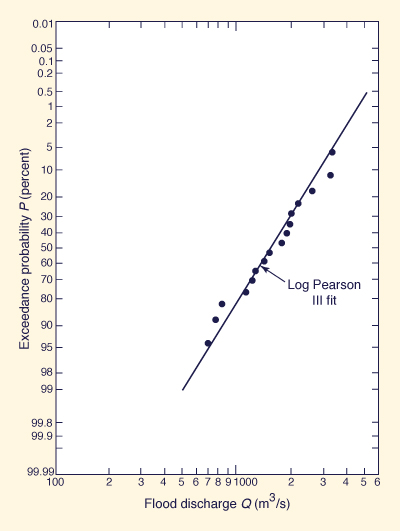
Plot the flood discharges Qj against probabilities Pj on log probability paper, with discharges in the log scale and probabilities in the probability scale.
The log Pearson III fit to the data is obtained by linking the points with a smooth curve.
For Csy = 0, the curve reduces to a straight line.
The procedure is illustrated by the following example.
Example 6-4.
Apply the log Pearson III method to the flood series of Example 6-3.
Plot the results on log probability paper along with the plotting positions calculated in Example 6-3.
The discharge values, Table 6-2, Col. 2, are converted to logarithms, and the mean, standard deviation, and skew coefficient of the logarithms calculated.
This results in ȳ = 3.187, sy = 0.207, and Csy = -0.116.
The computations are summarized in Table 6-3.
Column 1 shows selected return periods, and Col. 2 shows the associated probabilities in percent (exceedance probability).
Column 3 shows the frequency factors K for
ONLINE CALCULATION. Using ONLINE PEARSON,
the results are essentially the same, varying from Q = 691 m3/s for T = 1.05 y, to Q = 4984 m3/s for T = 200 y.
| |||||||||||||||||||||||||||||||||||||||||||||||||||||||||||||||||||||||
Figure 6-4 Log Pearson III fit: Example 6-4 [31]. |
Regional Skew Characteristics
The skew coefficient of the flood series (i.e., the station skew) is sensitive to extreme events.
The overall accuracy of the method is improved by using a weighted value of skew in lieu of the station skew.
First, a value of regional skew is obtained, and the weighted skew is calculated by weighing station and regional skews in inverse proportion to their mean square errors (MSE).
The formula for weighted skew is the following:
|
(MSE)sr Csy + (MSE)sy Csr Csw = ________________________________ (MSE)sr + (MSE)sy | (6-33) |
in which Csw = weighted skew; Csy = station skew; Csr = regional skew; (MSE)sy = mean square error of the station skew; and (MSE)sr = mean square error of the regional skew.
To develop a value of regional skew, it is necessary to assemble data from at least 40 stations or, alternatively, all stations within a 160-km radius.
The stations should have at least 25 y of record.
In certain cases, the paucity of data may require a relaxation of these criteria.
The procedure includes analysis by three methods: (1) skew isolines map, (2) skew prediction equation, and (3) statistics of station skews.
To develop a skew isolines map, each station skew is plotted on a map at the centroid of its catchment area, and the plotted data are examined to identify any geographic or topographic trends.
If a pattern is evident, isolines (lines of equal skew) are drawn and the MSE is computed.
The MSE is the mean of the square of the differences between observed skews and isoline skews.
If no pattern is evident, an isoline map cannot be developed, and this method is not considered further.
In the second method, a prediction equation is used to relate station skew to catchment properties and climatological variables.
The MSE is the mean of the square of the differences between observed and predicted skews.
In the third method, the mean and variance of the station skews are calculated.
In some cases, the variability of runoff may be such that all the stations may not be hydrologically homogeneous.
If this is the case, the values of about 20 stations can be used to calculate the mean and variance of the data.
Of the three methods, the one providing the most accurate estimate of skew coefficient is selected.
First a comparison of the MSEs from the isolines map and prediction equations is made.
Then the smaller MSE is compared to the variance of the data.
If the smaller MSE is significantly smaller than the variance, it should be used in Eq. 6-33 as (MSE)sr.
If this is not the case, the variance should be used as (MSE)sr, with the mean of the station skews used as regional skew (Csr).
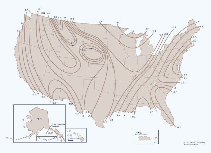
In the absence of regional skew studies, generalized values of regional skew for use in Eq. 6-33 can be obtained from Fig. 6-5.
When regional skew is obtained from this figure, the mean square error of the regional skew is MSEsr = 0.302.
The mean square error of the station skew is approximated by the following formula:
| (MSE)sy = 10 A - B log (n/10) | (6-34) |
in which
| A = - 0.33 + 0.08G, for G < 0.9 | (6-34a) |
| A = 0.52 + 0.30G, for G ≥ 0.9 | (6-34b) |
| B = 0.94 - 0.26G, for G < 1.5 | (6-34c) |
| B = 0.55, for G ≥ 1.5 | (6-34d) |
with G = absolute value of the station skew, and n = record length in years.
Figure 6-5 Generalized skew coefficient of logarithms of annual maximum streamflow [31] (Click -here- to display). |
Example 6-5.
A station in San Diego, California, has flood records for 34 y, with station skew Csy = - 0.1.
Calculate a weighted skew following Eq. 6-33 and Fig. 6-5.
From Fig. 6-5, the generalized value of regional skew is Csr = -0.3.
The MSE of the station skew is calculated by Eq. 6-34, with G = 0.1: (MSE)sy = 0.156.
Therefore, the weighted skew is (Eq. 6-33):
|
Treatment of Outliers
Outliers are data points that depart significantly from the overall trend of the data.
The treatment of these outliers (i.e., their retention, modification, or deletion) may have a significant effect on the value of the statistical parameters computed from the data, particularly for small samples.
Procedures for treatment of outliers invariably require judgment involving mathematical and hydrologic considerations.
The detection and treatment of high and low outliers in the log Pearson III method is performed in the following way [31].
For station skew greater than +0.4, tests for high outliers are considered first.
For station skew less than -0.4, tests for low outliers are considered first.
For station skew in the range -0.4 to +0.4, tests for high and low outliers are considered simultaneously, without eliminating any outliers from the data.
The following equation is used to detect high outliers:
| yH = ȳ + Kn sy | (6-35) |
in which yH = high outlier threshold (in log units); and Kn = outlier frequency factor, a function of record length n.
Values of yH are given in Table A-7 (Appendix A).
Values of yi (logarithms of the flood series) greater than yH are considered to be high outliers.
If there is sufficient evidence to indicate that a high outlier is a maximum in an extended period of time, it is treated as historical data.
Otherwise, it is retained as part of the flood series.
Historical data refers to flood information outside of the flood series, which may be used to extend the record to a period much longer than that of the flood series.
Historical knowledge is used to define the historical period H, which is longer than the record period n.
The number z of events that are known to be the largest in the historical period are given a weight of 1.
The remaining n events from the flood series are given a weight of (H - z)/n.
For instance, for a record length n = 44 y, a historical period H = 77 y, and a number of peaks in the historical period z = 3, the weight applied to the three historical peaks would be 1, and the weight applied to the remaining flood series would be (77 - 3)/44 = 1.68.
In other words, the record is extended to 77 y, and the 44 y of flood series (excluding outliers that have been considered part of the historical data) represent 74 y of data in the historical period of 77 y [31].
The following equation is used to detect low outliers:
| yL = ȳ - Kn sy | (6-36) |
in which yL = low outlier threshold (in log units) and other terms are as defined previously.
If an adjustment for historical data has been previously made, the values on the right-hand side of Eq. 6-36 are those previously used in the historically weighted computation.
Values of yi smaller than yL are considered to be low outliers and deleted from the flood series [31].
Complements to Flood Frequency Estimates
The accuracy of flood estimates based on frequency analysis deteriorates for values of probability much greater than the record length.
This is due to sampling error and to the fact that the underlying distribution is not known with certainty.
Alternative procedures that complement the information provided by flood frequency analysis are recommended.
These procedures include flood estimates from precipitation data (e.g., unit hydrograph, Chapter 5) and comparison with catchments of similar hydrologic characteristics (regional analysis, Chapter 7).
Table 6-4 shows the relationship between the various types of analysis used in flood frequency studies.
| |||||||||||||||||||||||
Gumbel's Extreme Value Type I Method
The extreme value Type I distribution, also known as the Gumbel method [16], or EVl, has been widely used in the United States and other countries.
The method is a special case of the three-parameter GEV distribution described in the British Flood Studies Report [23].
The cumulative density function F(x) of the Gumbel method is the double exponential, Eq. 6-19, repeated here for convenience:
| F(x) = e -e -y | (6-19) |
in which F(x) is the probability of nonexceedance.
In flood frequency analysis, the probability of interest is the probability of exceedance, i.e., the complementary probability to F(x):
| G(x ) = 1 - F(x ) | (6-37) |
The return period T is the reciprocal of the probability of exceedance.
Therefore,
|
1 _____ = 1 - e -e -y T | (6-38) |
From Eq. 6-38:
|
T y = - ln ln _______ T - 1 | (6-39) |
In the Gumbel method, values of flood discharge are obtained from the frequency formula, Eq. 6-29, repeated here for convenience:
| x = x̄ + K s | (6-29) |
The frequency factor K is evaluated with the frequency formula:
| y = ȳn + K σn | (6-40) |
in which y = Gumbel (reduced) variate, a function of return period (Eq. 6-39); and ȳn and σn are the mean and standard deviation of the Gumbel variate, respectively.
These values are a function of record length n (see Table A-8, Appendix A).
In Eq. 6-29, for K = 0, x is equal to the mean annual flood x̄.
Likewise, in Eq. 6-40, for K = 0, the Gumbel variate y is equal to its mean ȳn.
The limiting value of ȳn, for n → ∞ is the Euler constant, 0.5772 [28].
In Eq. 6-38, for y = 0.5772: T = 2.33 years.
Therefore, the return period of 2.33 y is taken as the return period of the mean annual flood.
From Eqs. 6-29 and 6-40:
|
y - ȳn x = x̄ + ___________ s σn | (6-41) |
and with Eq. 6-39:
|
ln ln [T / (T - 1)] + ȳn x = x̄ + __________________________ s σn | (6-42) |
The following steps are necessary to apply the Gumbel method:
Assemble the flood series.
Calculate the mean x̄ and standard deviation s of the flood series.
Use Table A-8 to determine the mean ȳn and standard deviation σn of the Gumbel variate as a function of record length n.
Select several return periods Tj and associated exceedance probabilities Pj.
Calculate the Gumbel variates yj corresponding to the return periods Tj by using Eq. 6-39, and calculate the flood discharge Qj = xj for each Gumbel variate (and associated return period) using Eq. 6-41. Alternatively, the flood discharges can be calculated directly for each return period by using Eq. 6-42.
Values of Q are plotted against y or T (or P) on Gumbel probability paper, and a straight line is drawn through the points.
Gumbel probability paper has an arithmetic scale of Gumbel variate y in the abscissas and an arithmetic scale of flood discharge Q in the ordinates.
To facilitate the reading of frequencies and probabilities, Eq. 6-38 may be used to superimpose a scale of return period T (or probability P) on the arithmetic scale of Gumbel variate y.
Example 6-6.
Apply the Gumbel method to the flood series of Example 6-3.
Plot the results on Gumbel paper along with the plotting positions calculated in Example 6-3.
The mean and standard deviation of the flood series are: x̄ = 1704 m3/s and s = 795 m3/s.
From Table A-8. for n = 16, the mean and standard deviation of the Gumbel variate are ȳ = 0.5157 and σn = 1.0316.
The results are shown in Table 6-5.
Columns 1 and 2 show selected return periods T and associated exceedance probabilities (in percent).
Column 3 shows the values of Gumbel variate calculated by Eq. 6-39.
Column 4 shows the flood discharge Q calculated by Eq. 6-41 for each variate y, return period T, and associated exceedance probability P.
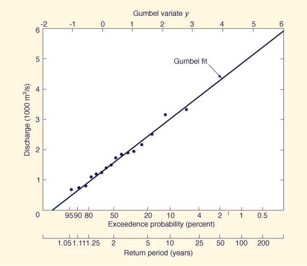
The flood discharges define a straight line when plotted versus return period on Gumbel paper, as shown by the solid line of Fig. 6-6. Plotting positions calculated by Example 6-3 are shown for comparison purposes.
ONLINE CALCULATION. Using ONLINE GUMBEL,
the results are essentially the same, varying from Q = 447 m3/s for T = 1.05 y, to Q = 5396 m3/s for T = 200 y.
| |||||||||||||||||||||||||||||||||||||||||||||||||||||||||
Figure 6-6 Flood frequency analysis by Gumbel method: Example 6-6. |
Modifications to the Gumbel Method
Since its inception in the 1940s, several modifications to the Gumbel method have been proposed.
Gringorten [12] has shown that the Gumbel distribution does not follow the Weibull plotting rule, Eq. 6- 26 (or Eq. 6-27 with a = 0).
He recommended a = 0.44, which led to the Gringorten plotting position formula:
|
1 m - 0.44 ____ = P = _______________ T n + 0.12 | (6-43) |
Lettenmaier and Burges [22] have suggested that better flood estimates are obtained by using the limiting values of mean and standard deviation of the Gumbel
variate (i.e., those corresponding to
In this case, ȳn = 0.5772, and σn = π / 61/2 = 1.2825.
Therefore, Eq. 6-41 reduces to
| x = x̄ + (0.78 y - 0.45) s | (6-44) |
and Eq. 6-42 reduces to
|
T x = x̄ + (0.78 ln ln _______ + 0.45) s T - 1 | (6-45) |
Lettenmaier and Burges [22] have also suggested that a biased variance estimate, using n as the divisor in Eq. 6-3, yields better estimates of extreme events that the usual unbiased estimate, that is, the divisor n - 1.
Comparison Between Flood Frequency Methods
In 1966, the Hydrology Subcommittee of the U.S. Water Resources Council began work on selecting a suitable method of flood frequency analysis that could be recommended for general use in the United States.
The committee tested the goodness of fit of six distributions: (1) lognormal, (2) log Pearson III, (3) Hazen, (4) gamma, (5) Gumbel (EV1) and (6) log Gumbel (EV2).
The study included ten sets of records, the shortest of which was 40 y.
The findings showed that the first three distributions had smaller average deviations that the last three.
Since the Hazen distribution is a type of lognormal distribution and the lognormal is a special case of the log Pearson III, the Committee concluded that the latter was the most appropriate of the three, and hence recommended it for general use.
The same type of analysis was repeated for six sets of records in the United Kingdom, the shortest of which was 32 y [2].
The methods were: (1) gamma, (2) log gamma, (3) lognormal, (4) Gumbel (EV1), (5) GEV, (6) Pearson Type III, and (7) log Pearson III.
At low return periods (from 2 to 5 y), the GEV and Pearson Type III showed the smallest average deviations, whereas for return periods exceeding 10 y the log Pearson III method had the smallest average deviations.
Similar comparative studies were reported in the British Flood Studies Report [23].
The study concluded that the three-parameter distributions (GEV, Pearson Type III, and log Pearson III) provided a better fit than the two-parameter distributions (Gumbel, lognormal, gamma, log gamma).
Based on mean absolute deviation criteria, the study rated the log Pearson III method better than the GEV and the latter better than the Pearson Type III.
However, based on root mean square deviation, it rated the Pearson Type III better than both the log Pearson III and GEV distributions.
Although in general, the three-parameter methods seemed to fare better than the two-parameter methods, the latter should not be completely discarded.
The British Flood Studies Report [23] observed that their use in connection with short record lengths often leads to results which are more sensible than those obtained by fitting three-parameter distributions.
A three-parameter distribution fitted to a small sample may in some cases imply that there is an upper bound to the flood discharge equal to about twice the mean annual flood.
While there may be an upper limit to flood magnitude, it is certainly higher than twice the mean annual flood.
6.3 LOW-FLOW FREQUENCY
|
|
Whereas high flows lead to floods, sustained low flows can lead to droughts.
A drought is defined as a lack of rainfall so great and continuing so long as to affect the plant and animal life of a region adversely and to deplete domestic and industrial water supplies, especially in those regions where rainfall is normally sufficient for such purposes [18].
In practice, a drought refers to a period of unusually low water supplies, regardless of the water demand.
The regions most subject to droughts are those with the greatest variability in annual rainfall.
Studies have shown that regions where the variance coefficient of annual rainfall exceeds 0.35 are more likely to have frequent droughts [6].
Low annual rainfall and high annual rainfall variability are typical of arid and semiarid regions.
Therefore, these regions are more likely to be prone to droughts.
Studies of tree rings, which document long term trends of rainfall, show clear patterns of periods of wet and dry weather [30].
While there is no apparent explanation for the cycles of wet and dry weather, the dry years must be considered in planning water resource projects.
Analysis of long records has shown that there is a tendency for dry years to group together.
This indicates that the sequence of dry years is not random, with dry years tending to follow other dry years.
It is therefore necessary to consider both the severity and duration of a drought period.
The severity of droughts can be established by measuring:
The deficiency in rainfall and runoff,
The decline of soil moisture, and/or
The decrease in groundwater levels.
Alternatively, low-flow-frequency analysis can be used in the assessment of the probability of occurrence of droughts of different durations.
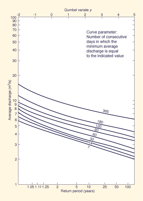
Figure 6-7 Low-flow frequency curves [28]. |
Methods of low-flow frequency analysis are based on an assumption of invariance of meteorological conditions.
The absence of long records, however, imposes a stringent limitation on low-flow frequency analysis.
When records of sufficient length are available, analysis begins with the identification of the low-flow series.
Either the annual minima or the annual exceedance series are used.
In a monthly analysis, the annual minima series is formed by the lowest monthly flow volumes in each year of record.
If the annual exceedance method is chosen, the lowest monthly flow volumes in the record are selected, regardless of when they occurred.
In the latter method, the number of values in the series need not be equal to the number of years of record.
A flow duration curve can be used to give an indication of the severity of low flows.
Such a curve, however, does not contain information on the sequence of low flows or the duration of possible droughts.
The analysis is made more meaningful by abstracting the minimum flows over a period of several consecutive days.
For instance, for each year, the 7-day period with minimum flow volume is abstracted, and the minimum flow is the average flow rate for that period.
A frequency analysis on the low-flow series, using the Gumbel method, for instance, results in a function describing the probability of occurrence of low flows of a certain duration.
The same analysis repeated for other durations leads to a family of curves depicting low-flow frequency, as shown in Fig. 6-7 [28].
In reservoir design, the assessment of low flows is aided by a flow-mass curve.
The technique involves the determination of storage volumes required for all low-flow periods.
Although it is practically impossible to provide sufficient storage to meet hydrologic risks of great rarity, common practice is to provide for a stated risk (i.e., a drought probability) and to add a suitable percent of the computed storage volume as reserve storage allowance.
The variance coefficient of annual flows is used in determining the risk and storage allowance levels.
Extraordinary drought levels are then met by cutting draft rates.
Regulated rivers may alter natural flow conditions to provide a minimum downstream flow for specific purposes.
In this case, the reservoirs serve as the mechanism to diffuse the natural flow variability into downstream flows which can be made to be nearly constant in time.
Regulation is necessary for downstream low-flow maintenance, usually for the purpose of meeting agricultural, municipal and industrial water demands, minimum instream flows, navigation draft, and water pollution control regulations.
6.4 DROUGHTS
|
|
Drought is a weather-related natural phenomenon, affecting regions of the Earth for months or years.
It has an impact on food production, reducing life expectancy and the economic performance of large geographic regions or entire countries.
Drought is a recurrent feature of the climate; it occurs in virtually all climatic zones, with its characteristics varying significantly among regions.
Drought differs from aridity in that drought is temporary; aridity is a permanent characteristic of regions with low rainfall.
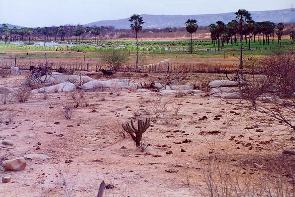
Drought is related to a deficiency of precipitation over an extended period of time, usually for a season or more (Fig. 6-8).
This deficiency results in a water shortage for some activity, group, or environmental sector.
Drought is also related to the timing of precipitation.
Other climatic factors such as high temperature, high wind, and low relative humidity are often associated with drought.
Drought is more than a physical phenomenon or natural event.
Its impact results from the relation between a natural event and the demands on the water supply, and it is often exacerbated by human activities.
The experience from droughts has underscored the vulnerability of human societies to this natural hazard.
Figure 6-8 Backlands in Rio Grande do Norte, in the drought-stricken Brazilian Northeast. |
Definition of drought
Drought definitions are of two types: (1) conceptual, and (2) operational.
Conceptual definitions help understand the meaning of drought and its effects.
For example, drought is a protracted period of precipitation deficiency which causes extensive damage to crops, resulting in loss of yield.
Operational definitions help identify the drought's beginning, end, and degree of severity.
To determine the beginning of drought, operational definitions specify the degree of departure from the precipitation average over some time period.
This is usually accomplished by comparing the current situation (the study period) with the historical average.
The threshold identified as the beginning of a drought (e.g., 75% of average precipitation over a specified time period) is usually established somewhat arbitrarily.
An operational definition for agriculture may compare daily precipitation to evapotranspiration to determine the rate of soil-moisture depletion, and express these relationships in terms of drought effects on plant behavior.
Operational definitions are used to analyze drought frequency, severity, and duration for a given historical period.
Such definitions, however, require weather data on hourly, daily, monthly, or other time scales and, possibly, impact data (e.g., crop yield).
A climatology of drought for a given region provides a greater understanding of its characteristics and the probability of recurrence at various levels of severity.
Information of this type is beneficial in the formulation of mitigation strategies.
Types of droughts
The following types of drought have been identified:
- Meteorological drought,
- Agricultural drought,
- Hydrological drought, and
- Socieoeconomic drought.
Meteorological drought is defined on the basis of the degree of dryness, in comparison to a normal or average amount, and the duration of the dry period.
Definitions of meteorological drought must be region-specific, since the atmospheric conditions that result in deficiencies of precipitation are highly variable.
The variety of meteorological definitions in different countries illustrates why it is not possible to apply a definition of drought developed in one part of the world to another.
For instance, the following definitions of drought have been reported:
United States (1942): Less than 2.5 mm of rainfall in 48 hours.
Great Britain (1936): Fifteen consecutive days with daily precipitation less than 0.25 mm.
Libya (1964): When annual rainfall is less than 180 mm.
Bali (1964): A period of six days without rain.
Data sets required to assess meteorological drought are: (1) daily rainfall, (2) temperature, (3) humidity, (4) wind velocity, and (5) evaporation.
Agricultural drought links various characteristics of meteorological drought to agricultural impacts, focusing on precipitation shortages, differences between actual and potential evapotranspiration, soil-water deficits, reduced groundwater or reservoir levels, and so on.
Plant water demand depends on prevailing weather conditions, biological characteristics of the specific plant, its stage of growth, and the physical and biological properties of the soil.
A good definition of agricultural drought should account for the susceptibility of crops during different stages of crop development.
Deficient topsoil moisture at planting may hinder germination, leading to low plant populations per hectare and a reduction of yield.
Data sets required to assess agricultural drought are: (1) soil texture, (2) soil fertility, (3) soil moisture, (4) crop type and area, (5) crop water requirements, (6) pests, and (7) climate.
Hydrological drought refers to a persistently low discharge and/or volume of water in streams and reservoirs, lasting months or years.
Hydrological drought is a natural phenomenon, but it may be exacerbated by human activities.
Hydrological droughts are usually related to meteorological droughts, and their recurrence interval varies accordingly.
Changes in land use and land degradation can affect the magnitude and frequency of hydrological droughts.
Data sets required to assess hydrological drought are: (1) surface-water area and volume, (2) surface runoff, (3) streamflow measurements, (4) infiltration, (5) water-table fluctuations, and (6) aquifer properties.
Socioeconomic drought associates the supply and demand of some economic good with elements of meteorological, hydrological, and agricultural drought.
It differs from the other types of drought in that its occurrence depends on the processes of supply and demand.
The supply of many economic goods, such as water, forage, food grains, fish, and hydroelectric power, depends on the weather.
Due to the natural variability of climate, water supply is ample in some years but insufficient to meet human and environmental needs in other years.
Socioeconomic drought occurs when the demand for an economic good exceeds the supply as a result of a weather-related shortfall in water supply.
The drought may result in significantly reduced hydroelectric power production because power plants were dependent on streamflow rather than storage for power generation.
Reducing hydroelectric power production may require the government to convert to more expensive petroleum alternatives and to commit to stringent energy conservation measures to meet its power needs.
The demand for economic goods is increasing as a result of population growth and economic development.
The supply may also increase because of improved production efficiency, technology, or the construction of reservoirs.
When both supply and demand increase, the critical factor is their relative rate of change.
Socioeconomic drought is promoted when the demand for water for economic activities far exceeds the supply.
Data sets required to assess socioeconomic drought are: (1) human and animal population, (2) growth rate, (3) water and fodder requirements, (4) severity of crop failure, and (5) industry type and water requirements.
Intensity-Duration-Frequency Relations
The relations between intensity, duration, and frequency of droughts may be analyzed by the conceptual model described in Table 6-6 [27].
The conceptual approach is applicable to meteorological droughts lasting at least one year, in midlatitudinal regions where the prevailing climate may be primarily characterized by precipitation.
The climate types, from superarid to superhumid, are defined in terms of mean annual precipitation Pma (mm) as shown in Table 6-6, Line 1:
|
The (mean) annual global terrestrial precipitation is Pagt = 800 mm [27].
At the extremes of the climatic spectrum, mean annual precipitation is less than 100 mm (superarid), or greater than 6400 mm (superhumid).
The superarid example is the Atacama desert, in northern Chile, with mean annual precipitation Pma = 0.5 mm, which is hardly measurable.
The superhumid example is Cherrapunji, in Meghalaya, Esatern India, with mean annual precipitation Pma = 11,777 mm, long considered by many as the wettest spot on Earth.
However, Mawsynran, near Cherrapunji, now boasts Pma = 11,873 mm, effectively edging out Cherrapunji of the distinction.
Climates types may also be defined as the ratio of mean annual precipitation Pma to (mean) annual global terrestrial precipitation Pagt (Line 2).
The ratio Pma/Pagt = 1 depicts the middle of the climatic spectrum.
The conceptual model is also defined in terms of the annual potential evaporation (evapotranspiration) Eap (Line 3) and of the ratio of annual potential evaporation to mean annual precipitation Eap/Pma (Line 4).
The ratio Eap/Pma = 2 describes the middle of the climatic spectrum.
To complement the description, the length of the rainy season Lrs is also indicated (Line 5).
| ||||||||||||||||||||||||||||||||||||||||||||||||||||||||||||||||||||||||||||||||||||||||||||||||||||||||||||||||||||||
For any year for which P is the annual precipitation, drought intensity I is defined as the ratio of the deficit (Pma - P) to the mean (Pma).
For any year, an intensity I = 0.25 is classified as moderate;
For drought durations lasting two years or more, intensity is the summation of the individual annual intensities (Lines 6-8, Table 6-6).
Therefore, the longer the drought duration, the greater the drought intensity.
Extreme intensities are generally associated with droughts of long duration.
Experience has shown that the longer droughts generally occur around the middle of the climatic spectrum (800 mm of mean annual precipitation).
Drought duration varies between 1 yr (or less) at the extremes of the climatic spectrum and (about) 6 yr around the middle (Line 9) [26].
Droughts lasting more than 6 yr are uncommon; they are more likely to be driven by anthropogenic pressures, for instance, deforestation or overgrazing [25].
A classical example of an anthropogenically derived drought is that of the Sahel, in Northern Africa (Fig. 6-9), where, in the past 40 years, droughts have had a tendency to persist for durations much longer than normal.
Figure 6-10 shows values of standardized annual seasonal rainfall (June-October) in the Sahel for the period 1898-2004.
The standardized annual rainfall has zero mean and unit standard deviation.
Note that through the 1980s, drought in the Sahel persisted for more than 10 years.
|
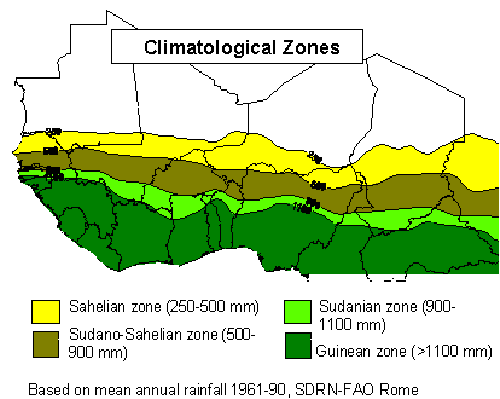
Figure 6-9 Mean annual precipitation in the Sahel, North Africa.
Figure 6-10 Standardized annual rainfall in the Sahel for the period 1898-2004. |
In general, the dry periods (drought events) are followed by corresponding wet periods.
Therefore, the drought recurrence interval (i.e., the reciprocal of the frequency) is always greater than the drought duration.
Drought recurrence intervals increase from 2 year on the extreme dry side of the climatic spectrum (superarid) to (more than) 100 years on the extreme wet side (superhumid) (Line 10, Table 6-6).
QUESTIONS
|
|
In statistical analysis, what are the measures of central tendency? Explain.
What is skewness? A distribution with a long tail on the right side has positive or negative skewness?
What are the parameters of the gamma distribution? How are the gamma and Pearson Type III distributions related?
What is the parameter that distinguishes the three extreme value distributions? What is the limiting value of the mean of the Gumbel variate?
What is the difference between the annual exceedance series and the annual maxima series? What is risk in the context of frequency analysis?
How is an extreme value probability paper constructed? What type of probability paper is used in the log Pearson Type III method?
What is the difference between the Weibull, Blom, and Gringorten plotting position formulas?
How is skewness variability accounted for in the log Pearson III method?
When are high outliers considered part of historical data? When is it necessary to perform a historically weighted computation?
Why are two-parameter distributions such as the Gumbel distribution appropiate for use in connection with short record lengths?
Compare floods and droughts from the standpoint of frequency analysis.
What is the mean annual precipitation in the middle of the climatic spectrum?
What is the mean annual evaporation in the middle of the climatic spectrum?
Why are the droughts in the Sahel likely to persist much longer than normal?
PROBLEMS
|
|
Develop a spread sheet to calculate the mean, standard deviation, and skew coefficient of a series of annual maximum flows. Test your work using the data of Example 6-1 in the text.
The annual maximum flows of a certain stream have been found to be normally distributed with mean 22,500 ft3/s and standard deviation 7500 ft3/s. Calculate the probability that a flow larger than 39,000 ft3/s will occur.
The 10-y and 25-y floods of a certain stream are 73 and 84 m3/s, respectively. Assuming a normal distribution, calculate the 50-y and 100-y floods.
The low flows of a certain stream have been shown to follow a normal distribution. The flows expected to be exceeded 95% and 90% of the time are 15 and 21 m3/s, respectively. What flow can be expected to be exceeded 80% of the time?
A temporary cofferdam for a 5-y dam construction period is designed to pass the 25-y flood. What is the risk that the cofferdam may fail before the end of the construction period? What design return period is needed to reduce the risk to less than 10%?
Use the Weibull formula (Eq. 6-26) to calculate the plotting positions for the following series of annual maxima, in cubic feet per second: 1305, 3250, 4735, 5210, 4210, 2120, 2830, 3585, 7205, 1930, 2520, 3250, 5105, 4830, 2020, 2530, 3825, 3500, 2970, 1215.
Use the Gringorten formula to calculate the plotting positions for the following series of annual maxima, in cubic meters per second: 160, 350, 275, 482, 530, 390, 283, 195, 408, 307, 625, 513.
Modify the spread sheet of Problem 6-1 to calculate the mean, standard deviation, and skew coefficients of the logarithms of a series of annual maximum flows. Test your work using the results of Example 6-4 in the text.
Fit a log Pearson III curve to the data of Problem 6-6. Plot the calculated distribution on log probability paper, along with the Weibull plotting positions calculated in Problem 6-6.
Fit a Gumbel curve to the data of Problem 6-6. Plot the calculated distribution on Gumbel paper, along with the Weibull plotting positions calculated in Problem 6-6.
Develop a spread sheet to read a series of annual maxima, sort the data in descending order, and compute the corresponding plotting positions (percent chance and retum period) by the Weibull and Gringorten formulas.
Given the following statistics of annual maxima for stream X: number of years n = 35;
mean = 3545 ft3/s ; standard deviation = 1870 ft3/s. Compute the 100-y flood by the Gumbel method.Given the following statistics of annual maxima for river Y: number of years n = 45;
mean = 2700 m3/s ; standard deviation 1300 m3/s; mean of the logarithms = 3.1; standard deviation of the logarithms = 0.4; skew coefficient of the logarithms = - 0.35. Compute the 100-y flood using the following probability distributions: (a) normal, (b) Gumbel, and (c) log Pearson III.A station near Denver, Colorado, has flood records for 48 y, with station skew
Csy = - 0.18. Calculate a weighted skew coefficient.Determine if the value Q = 13,800 ft3/s is a high outlier in a 45-y flood series with the following statistics: mean of the logarithms = 3.572; standard deviation of the logarithms = 0.215.
Using the Lettenmaier and Burges modification to the Gumbel method, fit a Gumbel curve to the data of Example 6-6 in the text. Plot the calculated distribution on Gumbel paper, along with plotting positions calculated by the Gringorten formula.
REFERENCES
|
|
Benson, M. A. (1962). "Plotting Positions and Economics of Engineering Planning," Journal of the Hydraulics Division, ASCE, Vol. 88, November, pp. 57-71.
Benson, M. A. (1968). "Uniform Flood Frequency Estimating Methods for Federal Agencies," Water Resources Research, Vol. 4, pp. 891-908.
Blom, G. (1958). Statistical Estimates and Transformed Beta Variables. New York: John Wiley.
Casella, G., and R. L. Berger. (1990). Statistical Inference, Wadsworth & Brooks/Cole, Pacific Grove, California.
Chow, V. T. (1951). "A General Formula for Hydrologic Frequency Analysis," Transactions, American Geophysical Union, Vol. 32, pp. 231-237.
Chow, V. T. (1964). Handbook of Applied Hydrology. New York: McGraw-Hill.
Cunnane, C. (1978). "Unbiased Plotting Positions-A Review," Journal of Hydrology, Vol. 37, pp. 205-222.
Fisher, R. A., and L. H. C. Tippett. (1928). "Limiting Forms of a Frequency Distribution of the Smallest and Largest Member of a Sample," Proceedings, Cambridge Philosophical Society, Vol. 24, pp.180-190.
Foster, H. A. (1924). "Theoretical Frequency Curves and their Application to Engineering Problems," Transactions, ASCE, Vol. 87, pp. 142-173.
Frechet, M. (1927). "Sur la loi de Probabilite de l'ecart Maximum," (On the Probability Law of Maximum Error), Annals of the Polish Mathematical Society, (Cracow), Vol. 6, pp. 93-116.
Fuller, W. E. (1914). "Flood Flows," Transactions, ASCE, Vol. 77, pp. 564-617.
Gringorten, 1.1. (1963). "A Plotting Rule for Extreme Probability Paper," Journal of Geophysical Research, Vol. 68, No.3, February, pp. 813-814.
Gumbel, E. J. (1941). "Probability Interpretation of the Observed Return Periods of Floods," Transactions, American Geophysical Union, Vol. 21, pp. 836-850.
Gumbel, E. J. (1942). "Statistical Control Curves for Flood Discharges," Transactions, American Geophysical Union, Vol. 23, pp. 489-500.
K Gumbel , E. J. (1943). "On the Plotting of Flood Discharges," Transactions, American Geophysical Union, Vol. 24, pp. 699-719.
Gumbel, E. J. (1958). Statistics of Extremes. Irvington, N.Y.: Columbia University Press.
Hazen, A. (1914). Discussion on "Flood Flows," by W. E. Fuller, Transactions, ASCE, Vol. 77, p. 628.
Havens, A. V. (1954). "Drought and Agriculture," Weatherwise, Vol. 7, pp. 51-55.
Horton, R. E. (1913). "Frequency of Recurrence of Hudson River Floods," U.S. Weather Bureau Bulletin Z, pp. 109-112.
Jenkinson, A. F. (1955). "The Frequency Distributions of the Annual Maximum (or Minimum) Values of Meteorological Elements," Quarterly Journal of the Royal Meteorological Society, Vol. 87, p. 158.
Kite, G. W. (1977). Frequency and Risk Analyses in Hydrology. Fort Collins, Colorado: Water Resources Publications.
Lettenmaier, D. P., and S. J. Burges. (1982). "Gumbel's Extreme Value Distribution: A New Look," Journal of the Hydraulics Division, ASCE, Vol. 108, No. HY4, April, pp. 503-514.
Natural Environment Research Council. (1975). Flood Studies Report. Vol. 1 (of 5 volumes), London, England.
Pearson, K. (1930). "Tables for Statisticians and Biometricians," Part I, 3d. Ed. , The Biometric Laboratory, University College. London: Cambridge University Press.
Ponce, V. M., A. K. Lohani, and P. T. Huston. (1997). "Surface albedo and water resources: Hydroclimatological impact of human activities." Journal of Hydrologic Engineering, ASCE, Vol. 2, No. 4, October, 197-203.
Ponce, V. M., R. P. Pandey, and S. Ercan. (1999). "A conceptual model of drought characterization across the climatic spectrum." Revista de Estudos Ambientais, Vol. 1, No. 3, September-December, 68-76.
Ponce, V. M., R. P. Pandey, and S. Ercan. (2000). "Characterization of drought across climatic spectrum." Journal of Hydrologic Engineering, ASCE, Vol. 5, No. 2, April, 222-224.
Riggs, H. C. (1972). "Low-Flow Investigations," Techniques of Water Resources Investigations of the United States Geological Survey, Book 4, Chapter B1.
Spiegel, M. Mathematical Handbook of Formulas and Tables. Schaum's Outline Series in Mathematics. New York: McGraw-Hill.
Troxell, H. C. (1937). "Water Resources of Southern California with Special Reference to the Drought of 1944-51," U.S. Geological Survey Water Supply Paper No. 1366.
U.S. Interagency Advisory Committee on Water Data, Hydrology Subcommittee. (1983). "Guidelines for Determining Flood Flow Frequency," Bulletin No. 17B, issued 1981, revised 1983, Reston, Virginia.
Suggested Readings
Gumbel, E. J. (1958). Statistics of Extremes. Irvington, N.Y.: Columbia University Press.
Natural Environment Research Council. (1975). Flood Studies Report, in 5 volumes, London, England.
Riggs, H. C. (1972). "Low-Flow Investigations," Techniques of Water Resources Investigations of the United States Geological Survey, Book 4, Chapter B1.
U.S. Interagency Advisory Committee on Water Data, Hydrology Subcommittee. (1983). "Guidelines for Determining Flood Flow Frequency," Bulletin No. 17B, issued 1981, revised 1983, Reston, Virginia.
| http://engineeringhydrology.sdsu.edu |
|
150714 |