|
|
|
CHAPTER 4: HYDROLOGY OF SMALL CATCHMENTS |
|
"Roll waves are possible in the neighborhood of a uniform flow regime only when the Seddon celerity exceeds the Lagrange celerity." Antoine Craya (1952) |
|
This chapter deals with the hydrology of small catchments. It is divided into two sections. Section 4.1 describes the rational method and its application to urban storm drainage design. Section 4.2 discusses overland flow theory and applications. The choice of method is one scale, aided by individual preference and experience. |
4.1 RATIONAL METHOD
|
|
Small Catchments
A small catchment is described by the following features:
Storm rainfall can be assumed to be uniformly distributed in time,
Storm rainfall can be assumed to be uniformly distributed in space,
Storm duration typically exceeds time of concentration,
Runoff is primarily by overland flow, and
Channel slopes are steep enough so that channel storage processes are negligible.
A catchment possessing some or all of the above properties is small in a hydrologic sense.
Its runoff response may be described using relatively simple parametric or empirical methods, which lump all the relevant hydrologic processes into a few key descriptors such as rainfall intensity and catchment area.
When increased detail is required, small catchments may be analyzed using the more complex overland flow techniques, which can be either spatially lumped (the conceptual storage model, or storage concept) or distributed (a deterministic model of the kinematic or diffusion wave types).
For routine applications, all that is usually required is the simple parametric approach.
Exceptions may be warranted in certain specialized applications, e.g., when coupling water quantity and water quality models.
It is difficult to set the upper limit of a small catchment without being arbitrary to some degree.
Given the natural variability in catchment slopes, vegetation cover, and so on, no single value is universally applicable.
In practice, both time of concentration and catchment area have been used to define the upper limit of a small catchment.
Some authorities regard a catchment with a time of concentration of 1 h or less as a small catchment.
For others, a catchment of 2.5 km2 or less is considered small.
Any such limit is bound to be arbitrary, reflecting the accumulated body of experience in runoff response.
Rational Method
The rational method is the most widely used method for the analysis of runoff response from small catchments.
It has particular application in urban storm drainage, where it is used to calculate peak runoff rates for the design of storm sewers and small drainage facilities.
The popularity of the rational method is attributed to its simplicity, although reasonable care is necessary in order to use the method effectively.
The rational method takes into account the following hydrologic characteristics or processes:
- Rainfall intensity,
- Rainfall duration,
- Rainfall frequency,
- Catchment area,
- Hydrologic abstractions,
- Runoff concentration, and
- Runoff diffusion.
In general, the rational method provides only a peak discharge, although in the absence of runoff diffusion it is possible to obtain an isosceles-triangle-shaped runoff hydrograph.
The peak discharge is the product of:
- Runoff coefficient,
- Rainfall intensity, and
- Catchment area.
All processes are lumped into these three parameters.
Rainfall intensity contains information on rainfall duration and frequency.
In turn, rainfall duration is related to time of concentration, i.e., to the runoff concentration properties of the catchment.
The runoff coefficient accounts for hydrologic abstractions and runoff diffusion, and may also be used to account for frequency.
In this way, all the major hydrologic processes responsible for runoff response are embodied in the rational formula.
The rational method does not take into account the following characteristics or processes:
- Spatial or temporal variations in either total or effective rainfall,
- Time of concentration much greater than storm duration, and
- A significant portion of runoff occurring in the form of streamflow.
In addition, the rational method does not explicitly account for the catchment's antecedent moisture condition; however, the latter may be implicitly accounted for by varying the runoff coefficient.
The above conditions dictate that the rational method be restricted to small catchments.
To start, the assumption of constant rainfall in space and time can only be justified for small catchments.
Furthermore, in a small catchment, storm duration typically exceeds the time of concentration.
Finally, in a small catchment, surface runoff processes are usually dominated by overland flow.
There is no consensus regarding the upper limit of a small catchment.
Values ranging from 0.625 to 12.5 km2 have been quoted in the literature [2, 26].
The current trend is to use 1.25 to 2.5 km2 as the upper limit for the applicability of the rational method.
There is no theoretical lower limit, however, and catchments as small as 1 ha or less may be analyzed by the rational method.
The rational method is based on the following formula:
| Qp = C I A | (4-1) |
in which Qp = peak discharge corresponding to a given rainfall intensity, duration, and frequency; C = runoff coefficient, a dimensionless empirical coefficient related to the abstractive and diffusive properties of the catchment; I = rainfall intensity, averaged in time and space; and A = catchment area.
In SI Units, for rainfall intensity in millimeters per hour, catchment area in square kilometers, and peak discharge in cubic meters per second, the formula for the rational method is the following:
| Qp = 0.2778 C I A | (4-2) |
For rainfall intensity in millimeters per hour, catchment area in hectares, and peak discharge in liters per second, the formula is:
| Qp = 2.778 C I A | (4-3) |
In U.S. Customary units, for rainfall intensity in inches per hour, catchment area in acres, and peak discharge in cubic feet per second, the formula is:
| Qp = 1.008 C I A | (4-4) |
The unit conversion coefficient 1.008 is usually neglected on practical grounds.
Methodology
The first requirement of the rational method is that the catchment be small.
Once the size requirement has been met, the three components of the formula are evaluated.
The catchment area is determined by planimetering or other suitable means.
Boundaries may be established from topographic maps or aerial photographs.
The drainage area survey should also include:
Land use and land use changes,
Percentage of imperviousness,
Characteristics of soil and vegetative cover that may affect the runoff coefficient, and
General magnitude of ground slopes and catchment gradient necessary to determine time of concentration.
The evaluation of rainfall intensity is a function of several factors.
First, it is necessary to determine the time of concentration.
Normally, this is accomplished either:
By using an empirical formula,
By assuming a flow velocity based on hydraulic properties and calculating the travel time through the catchment's hydraulic length, or
By calculating the steady equilibrium flow velocity (using the Manning equation) and associated travel time through the hydraulic length.
Procedures to calculate time of concentration are not very well defined, often involving crucial assumptions such as flow level, channel shape, friction coefficients, and so on.
Nevertheless, a value of time of concentration can usually be developed for practical use.
For urban storm-sewer design, time of concentration at a point is the sum of two parts:
- Inlet time, and
- Time of flow in the storm sewer up to that point.
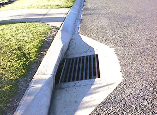
Inlet time is the longest time required for runoff to flow over the catchment surface to the nearest sewer inlet (Fig. 4-1).
Time of flow in the sewer, from inlet to point of interest, is calculated using hydraulic flow formulas.
Figure 4-1 Urban drainage inlet (University of Suth Queensland, Australia). |
Once time of concentration has been determined, the design storm duration is made equal to the time of concentration.
This amounts to an assumption of concentrated catchment flow (Section 2.4).
Subsequently, a rainfall frequency applicable to the given design condition is chosen.
Frequencies (and return periods) vary with the type of project and degree of protection desired.
Commonly used return periods are:
- 5 to 10 y for storm sewers in residential areas,
- 10 to 50 y for storm sewers in commercial areas, and
- 50 to 100 y for regional flood protection works.
The size and importance of the project, as well as design criteria established by federal, state and local agencies, have a bearing in the selection of design frequency.
The longer the return period (i.e., the smaller the frequency), the greater the peak discharge calculated by the rational formula.
Rainfall frequency versus peak flow frequency
The question of whether rainfall frequency and peak flow frequency are equivalent is an elusive one. The rational method bases the calculation of peak flow on a chosen rainfall frequency. In nature, however, the frequencies of storms and floods are not necessarily the same, largely due to the effect of antecedent moisture condition, variability in channel transmission losses, overbank storage, and the like. In practice, runoff coefficients are usually adjusted upward to reflect postulated decreases in runoff frequency. This procedure, while empirical, has seemed to work well.
Once rainfall duration and frequency have been determined, the corresponding rainfall intensity is obtained from the appropriate intensity-duration-frequency (IDF) curve.
An example of IDF curve is shown in Fig. 4-2.
The applicable curve can usually be obtained from cognizant government agencies.
Where IDF curves are nonexistent, they can be developed from regional isopluvial maps containing depth-duration-frequency data.
These maps are published by the National Weather Service [20, 21, 28].
Figure 4-2 An intensity-duration-frequency curve. |
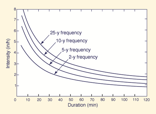
Due to the hyperbolic nature of the intensity-duration curve, an error in rainfall duration causes an error of opposite sign in rainfall intensity.
For instance, if the rainfall duration is too long (i.e., time of concentration too long), the calculated rainfall intensity will be too low, and vice versa.
Once rainfall intensity and catchment area have been obtained, a runoff coefficient applicable to the given design condition is selected.
Runoff coefficients are theoretically restricted in the range
In practice, values of runoff coefficient in the range 0.05 ≤ C ≤ 0.95 are usually adopted.
The runoff coefficient accounts for the processes of:
- Hydrologic abstractions, and
- Runoff diffusion.
In urban drainage design, hydrologic abstractions include interception, infiltration, and surface storage (Section 2.2).
Runoff diffusion is a measure of the catchment's ability to attenuate the flood peaks (Section 2.4).
In essence, the runoff coefficient is the ratio of the actual (calculated) peak runoff rate to the maximum possible runoff rate.
For C = 1, the calculated peak discharge is equal to the maximum possible discharge.
Typical values of runoff coefficients for a wide variety of conditions are given in design manuals and other reference books; see for instance Tables 4-1 (a) and (b).
These values reflect the reduction in peak runoff that is likely to be produced by a given combination of rainfall abstraction and runoff diffusion.
For instance, in Table 4-1 (a), a lawn with a steep gradient (greater than 7 percent) in a heavy (clayey) soil might have C = 0.3, but a lawn with a mild gradient (less than 2 percent) in a sandy soil might have C = 0.1, reflecting the prevailing abstractive and diffusive rates.
Furthermore, an asphaltic street (of negligible abstractive capability) might have
| ||||||||||||||||||||||||||||||||||||||||||||||||||||||||||||||||||||
The runoff coefficients shown in Table 4-1 (a) are applicable to storms of 5- to 10-y return period.
Less frequent storms (e.g., 50-y return period) require the use of higher coefficients because infiltration and other abstractions have a reduced role for the larger storms.
The coefficients shown in Table 4-1 (a) represent average antecedent moisture conditions and are not designed to account for multiple storms, or storms of very long duration.
Special design cases usually warrant the use of higher runoff coefficients to simulate the existence of wet antecedent moisture conditions in the catchment.
Experimental evidence has shown that runoff coefficients tend to increase from one storm to another occurring shortly
thereafter, with runoff coefficients tending to increase with storm duration.
| |||||||||||||||||||||||||||||||||||||||||||||||||||||||||||||||
Design values of runoff coefficients are usually a function of rainfall intensity and, therefore, of rainfall frequency.
Higher values of runoff coefficient are applicable for higher values of rainfall intensity and return period. A typical C versus I curve is shown in Fig. 4-3 [5].
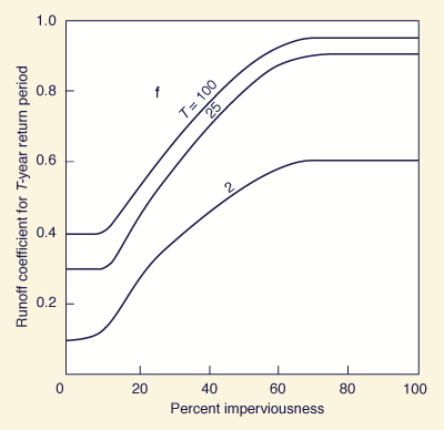
Alternate ways of expressing the variation of runoff coefficient with rainfall frequency are shown in Figs. 4-4 and 4-5 [6, 25].
Figure 4-3 Variation of runoff coefficient with rainfall intensity [5]. |
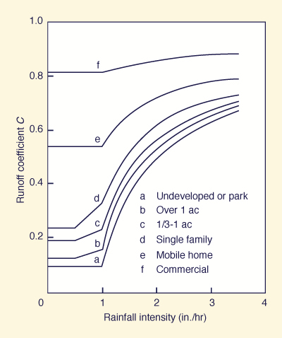
Figure 4-4 Variation of runoff coefficient with rainfall frequency [6]. |
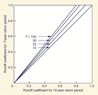
Figure 4-5 Variation of runoff coefficient with percent imperviousness and rainfall frequency [25]. |
With runoff coefficient, rainfall intensity, and catchment area determined, the peak discharge is calculated by Eq. 4-1.
The apparent simplicity of the procedure, however, is misleading.
For one thing, there is a range of possible runoff coefficients for each surface condition.
Therefore, the chosen C value is usually based on additional field information or designer's experience.
The effect of frequency and/or antecedent moisture condition needs to be evaluated carefully.
Furthermore, there is no absolute certainty that the calculated time of concentration (and, therefore, the rainfall duration) is correct, or even that it remains constant throughout the range of possible frequencies.
In fact, since larger flows generally travel with greater velocities (perhaps excepting the case of mild overbank flows, see Fig. 9-3), time of concentration tends to decrease with an increase in return period.
Notwithstanding these complexities, the rational method remains a practical way to calculate peak discharge for small catchments based on a few relevant parameters.
Example 4-1.
Calculate the peak flow Qp by the rational method for the following data: C = 0.6, I =
10 mm/h, and A = 15 ha (hectares).
The peak flow is:
Qp = C I A
Qp = ( 0.6 × 10 mm/h ×
0.001 m/mm × 15 ha × 10000 m2/ha × 1000 L/m3)
/ (3600 s/h) = 250 L/s.
ONLINE CALCULATION. Using the
RATIONAL online calculator,
the peak flow for the given data is: Qp = 250 L/s.
|
Theory of the Rational Method
The rational method is based on the principles of runoff concentration and diffusion.
For simplicity, the process can be explained in two parts:
- Concentration without diffusion, and
- Concentration with diffusion.
Runoff Concentration Without Diffusion
In the absence of diffusion, a catchment concentrates the flow at the outlet, attaining the maximum possible flow (i.e., the equilibrium flow rate) at the time of concentration.
By setting the design rainfall duration equal to the time of concentration, concentrated catchment flow is obtained at the outlet.
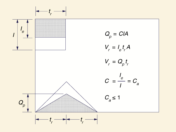
Since there is no diffusion, the method gives not only a peak flow but also a hydrograph corresponding to that of concentrated catchment flow (Fig. 4-6), with recession time equal to rising time.
The runoff coefficient is then simply the ratio of effective rainfall to total rainfall.
A mass balance of effective rainfall and runoff leads to:
| Vr = Ie tr A = C I A tr | (4-5) |
in which Vr = runoff volume; Ie = effective rainfall; and tr = rainfall duration (either effective or total). Equation 4-5 leads to:
Ie
|
C = Ca = ___ I | (4-6) |
in which Ca = runoff coefficient due only to abstraction (Ca ≤ 1).
Figure 4-6 Rational method: Flow concentration without diffusion. |
Runoff concentration without diffusion is typical of steep catchments, with slopes greater than 0.01, where the momentum balance is dominated by the gravitational and frictional forces.
For catchments of milder slope (say, less than 0.001), the role of the flow depth gradient increases, and runoff diffusion becomes increasingly important.
In the extreme case, for a hypothetical catchment of zero ground slope, the diffusion effect is theoretically the only one present.
Runoff Concentration With Diffusion
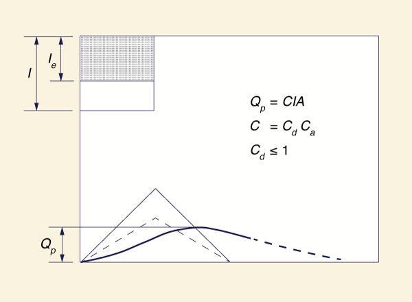
When diffusion is present, the rational method accounts for it in the runoff coefficient.
Thus, the runoff coefficient is used to model not only abstraction but also diffusion.
Diffusion modifies the catchment response in such a way as to increase the recession time and decrease the peak flow.
Therefore, a hydrograph shape can no longer be obtained directly from a mass balance as in the case of runoff concentration without diffusion.
The lack of a hydrograph shape does not impede the use of the rational method,
because the diffusion can be represented directly in the peak flow formula, by lowering the runoff
coefficient below that due only to abstraction
The reduction in the runoff coefficient amounts to:
| C = Cd Ca | (4-7) |
in which C = runoff coefficient and Cd = component of runoff coefficient accounting only for diffusion (Cd ≤ 1).
Figure 4-7 Rational method: Flow concentration with diffusion. |
The question of whether the peak is reached before, at, or after the time of concentration, as
In the absence of diffusion, Cd = 1 and C = Ca.
Likewise, in the absence of abstraction, Ca = 1 and
In the absence of abstraction and diffusion (e.g., a steep catchment with an impermeable surface): Ca = 1, Cd = 1, and, therefore, C = 1.
In practice, no quantitative distinction is made between the abstractive and diffusive components of the runoff coefficient.
Usage, however, reflects the fact that runoff diffusion is implicitly being considered; see, for instance, the marked change in runoff coefficient with surface slope shown in Table 4-1.
Further Developments
Attempts to analyze the behavior of the rational method have led to the concept of peak flow per unit area [27]:
Qp
|
qp = ____ = C I A | (4-8) |
in which qp = peak flow per unit area.
Rainfall intensity varies with rainfall duration and frequency.
Likewise, runoff coefficient also varies with rainfall duration and frequency.
Therefore, a relation linking peak flow per unit area to rainfall duration and frequency can be obtained:
| qp = f ( tr, T ) | (4-9) |
in which T = return period.
Another approach is based on expressing the rational formula in the following form:
Qp
|
C = _____ I A | (4-10) |
where now the runoff coefficient may be interpreted as dimensionless peak flow, or peak flow per unit area per unit rainfall intensity.
It follows that dimensionless peak flow is related to the abstractive and diffusive properties of the catchment.
A similar concept is used in the Natural Resources Conservation Service TR-55 method (Section 5.3).
In this method, a unit peak flow is defined as the peak flow per unit area per unit rainfall depth.
In the TR-55 graphical method included, the unit peak flow is a function of time of concentration, abstraction parameter, and temporal storm pattern.
The fact that unit peak flow is a function of temporal storm pattern qualifies the TR-55 graphical method as an extension of the rational method to midsize catchments.
While no upper limit to catchment size is indicated, the method is restricted to a time of concentration less than or equal to 10 h.
Applications of the Rational Method
Relation Between Runoff Coefficient and φ-index
The runoff coefficient can be related to total rainfall intensity and φ-index, provided the following assumptions are satisfied:
- Catchment response occurs under negligible diffusion, and
- Total and effective rainfall intensities are constant in time.
The first assumption is valid for steep catchments, whereas the second assumption is implicit in the application of the rational method.
For catchment response without diffusion:
Ie
|
C = Ca = ___ I | (4-11) |
For constant rainfall intensities:
| Ie = I - φ | (4-12) |
Combining Eqs. 4-11 and 4-12:
I - φ
|
C = _________ I | (4-13) |
Areal Weighing of Runoff Coefficients
Values of runoff coefficients may vary within a given catchment.
When a clear pattern of variation is apparent, a weighted value of runoff coefficient should be used.
For this purpose, the individual subareas are delineated and their respective runoff coefficients are identified.
The weighted value is obtained by weighing the runoff coefficients in proportion to their respective subareas.
This leads to:
|
Qp = 0.2778 I Σ ( Ci Ai ) i | (4-14) |
in which Ci = runoff coefficient of i th subarea and Ai = drainage area of i th subarea.
Applicable units are those of Eq. 4-2.
Composite Catchments
A composite catchment is one that drains two or more adjacent subareas of widely differing characteristics.
For instance, assume that a catchment has two subareas A and B with times of concentration tA and tB, respectively, with tA being much less than tB (Fig. 4-8).
Figure 4-8 Rational method: A composite catchment. |
To apply the rational method to this composite catchment, several rainfall durations are chosen, ranging from tA to tB in suitable increments.
The calculation proceeds by trial and error, with each trial associated with each rainfall duration.
To calculate the partial contribution from subarea B, an assumption must be made regarding the rate at which the flow is concentrated at the catchment outlet.
The rainfall duration that gives the highest combined peak flow (A plus B ) is taken as the design rainfall duration.
The procedure is illustrated by the following example.
Example 4-2.
Calculate the peak discharge by the rational method for a 1-km2 composite catchment with the following characteristics:
Assume a return period T = 10 y and the following IDF function:
1000T 0.2
in which I = rainfall intensity, in millimeters per hour; T = return period, in years; and tr = rainfall duration, in minutes.
To compute the contribution of subarea B, assume that the flow concentrates linearly at the outlet, i.e., each equal increment of time causes an equal increment of area contributing to the flow at the outlet.
First, choose rainfall durations between 20 min and 60 min at 10-min intervals.
For each rainfall duration, rainfall intensity is calculated by Eq. 4-15.
The assumption of linear concentration for subarea B leads to the following:
For tr = 20 min, the peak flow is (Eq. 4-14):
Successive trials for rainfall durations of 30, 40, 50, and 60 min result in lower peak flows.
Therefore, the peak flow is 9.986 m3/s and the design rainfall duration is 20 min.
ONLINE CALCULATION. Using the
ONLINE
RATIONAL COMPOSITE calculator,
the peak flow for the given data is: Qp = 9.9856 m3/s.
|
Effect of Catchment Shape
The rational method is suited to catchments where drainage area increases more or less linearly with catchment length.
If this is not the case, the peak flow may not increase with an increase in catchment area.
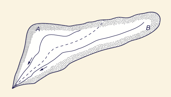
To illustrate, take the catchment shown in Fig. 4-9.
The time of concentration to point A is tA; the time of concentration to point B is tB; and tB is greater than tA.
Therefore, IA is greater than IB.
Figure 4-9 Rational method: Effect of catchment shape |
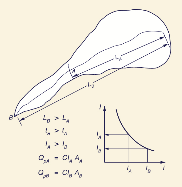
The drainage area to point A is AA, and the drainage area to point B is AB, and AB is greater than AA.
Assuming the same runoff coefficient for the partial area (to point A) and the total area (to point B), the peak flow at A is: QpA = CIAAA.
Likewise, the peak flow at B is: QpB = CIBAB.
For QpB to be greater than QpA, it is necessary that (AB / AA) be greater than (IA / IB).
In other words, the drainage area must grow in the downstream direction at least as fast as the decrease in corresponding rainfall intensity.
Otherwise, the peak discharge at A would be greater than that at B. The situation is illustrated by the following example.
Example 4-3.
Assume that the drainage area at A (Fig. 4-9) has a time of concentration such that the applicable rainfall intensity is 50 mm/h, and that from point A to point B the time of concentration increases, thereby decreasing the
applicable rainfall intensity for the drainage area at B to 40 mm/h.
Assume that the drainage area at A = 0.8 km2 and at B = 0.9 km2.
Compute the peak flow at points A and B. Assume C = 0.5.
The peak flow at A is (Eq. 4-2): QpA = 0.278 × 0.5 × 50 × 0.8 = 5.56 m3/s.
The peak flow at B is: QpB = |
Modified Rational Method
The application of the rational method to large urban catchments, i.e., those featuring well-defined conveyance channels and drainage areas greater than 1.3 km2 but less than 2.5 km2, requires special techniques.
For one thing, the flow is likely to vary widely along the main channel, ranging from small at the upstream reaches to larger at the downstream reaches.
In this case, it may be difficult to determine an average value of time of concentration.
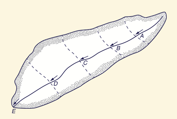
An alternative is to apply the rational method incrementally, using a technique known as the modified rational method.
The method requires the subdivision of the catchment into several subcatchments, as shown in Fig. 4-10.
First, the time of concentration tA is estimated and used to calculate the peak flow QpA at A, using Eq. 4-2.
With the aid of open channel flow formulas, QpA is conveyed through the main channel from A to B, and the travel time tAB calculated.
The time of concentration, tB = tA + tAB, is used to calculate the peak flow QpB at B, again using Eq. 4-2.
The procedure continues in the downstream direction until the peak flow QpE is calculated.
If the runoff coefficients are different for each subcatchment, Eq. 4-14 can be used in lieu of Eq. 4-2.
While the procedure is relatively straightforward, it may result in peak flows decreasing in the downstream direction (due to the effect of catchment shape).
Figure 4-10 Catchment subdivision in the modified rational method. |
Application to Storm-sewer Design
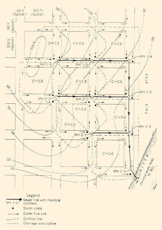
A typical plan for design of a small storm-sewer project is shown in Fig. 4-11.
Table 4-2 shows a summary of the computations illustrating the application of the rational method to determine design flows.
The example is based on the following conditions:
- Runoff Coefficients
- Resident area: C = 0.3
- Business area: C = 0.6
- Areal weighing of runoff coefficients where required.
- Intensity-Duration-Frequency curve shown in Fig. 2-12 (a). Selected design frequency: 5 y.
- Inlet time: 20 min.
- Manning n in sewer: 0.013.
- Free outfall to river at elevation 80.
-
A drop of 0.1 ft across each manhole where no change in pipe size occurs (to account for head losses).
When a change in pipe size occurs, set the elevation of 0.8 of pipe depths equal, and provide corresponding fall in manhole invert.
(Note: In larger systems, a more rigorous analysis of hydraulic losses through manholes, transitions, and changes in direction is required for adequate hydraulic design).
Figure 4-11 Typical storm-sewer design plan [2]. |
| ||||||||||||||||||||||||||||||||||||||||||||||||||||||||||||||||||||||||||||||||||||||||||||||||||||||||||||||||||||||||||||||||||||||||||||||||||||||||||||||||||||||||||||||||||||||||||||||||||||||||||||||||||||||||||||||||||||||||||||||||||||||||||||||||||||||||||||||||||||||||||||||||
This example is extracted from Design and Construction of Sanitary and Storm Sewers, ASCE Manual of Engineering Practice No. 37, 1960 [2].
4.2 OVERLAND FLOW
|
|
Overland flow is surface runoff that occurs in the form of sheet flow on the land surface without concentrating in clearly defined channels.
This type of flow is the first manifestation of surface runoff, since the latter occurs first as overland flow before it has a chance to flow into channels and become streamflow.
Overland flow theory uses deterministic methods to describe surface runoff in overland flow planes.
The theory is based on established principles of fluid mechanics such as laminar and turbulent flow, mass and momentum conservation, and unsteady free surface flow.
The spatial and temporal description leads to differential equations and to their solution by either analytical or numerical means.
For certain applications, simplified conceptual models can be developed for practical use.
Overland flow theory seeks to find an answer to the problem of catchment response: What is the hydrograph that will be produced at a catchment's outlet, subject to a given effective rainfall?
In overland flow applications, effective rainfall is also referred to as rainfall excess.
Unlike the rational method, which generally does not produce a hydrograph, overland flow models have the capability to account not only for runoff concentration but also for runoff diffusion.
Another advantage of overland flow models is their distributed nature, i.e., the fact that rainfall excess can be allowed to vary in space and time if necessary.
Overland flow models, then, are a more powerful tool than parametric models such as the rational method.
However, the complexity increases in direct relation to their greater level of detail.
As with the rational method, a question that must be addressed at the outset is the following: What size catchment can be analyzed with overland flow techniques?
Here again, the answer is not very well defined.
Intuitively, overland flow computations should be applicable to small catchments, primarily because overland flow is the main surface-flow feature of small catchments.
The method, however, is not necessarily restricted to small catchments.
Midsize catchments may also benefit from the increased detail of overland flow models.
The actual limit is a practical one.
Computations need to be performed in modules of relatively small size; otherwise, it is likely that the terrain's topographic, frictional, and vegetative features will not be properly represented in the overland flow model.
In practice, overland flow techniques are restricted to catchments for which the surface features can be adequately represented within the model's topological structure.
Otherwise, the amount of lumping introduced (i.e., temporal and spatial averaging) would interfere with the method's ability to predict the occurrence of flows in a distributed context.
Overland flow techniques often form part of computer models that simulate all relevant phases of the hydrologic cycle.
These models use overland flow techniques in their catchment routing component.
The fundamentals of overland flow theory are presented here.
Catchment routing methods are described in Chapter 10.
Overland Flow Theory
The mathematical description of overland flow begins with the equation of mass conservation of fluid mechanics, also referred to as the continuity equation.
In one-dimensional flow, this equation states that the change in flow per unit length
in a control volume is balanced by the change in fiow area per unit time:
∂Q ∂A
| ____ + ____ = 0 ∂x ∂t | (4-16) |
This equation does not include sources or sinks.
Inclusion of the latter leads to:
∂Q ∂A
| ____ + ____ =
qL ∂x ∂t | (4-17) |
in which qL = lateral inflow or outflow (inflow positive, outflow negative), or net lateral flow per unit length, in L2 T -1 units.
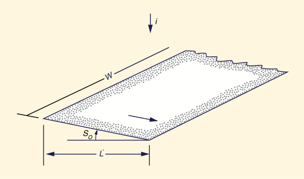
In small catchment hydrology, overland flow is assumed to take place on the overland flow plane.
This is a plane of length L (in the flow direction), slope So, and of sufficiently large width W (Fig. 4-12).
Therefore, a unit-width analysis is appropriate.
For a unit width, Eq. 4-17 is converted to:
∂q ∂h
| ____ + ____ =
i ∂x ∂t | (4-18) |
in which q = flow rate per unit width; h = flow depth; and i = lateral inflow (rainfall excess), or inflow per unit area, in L T -1 units.
While lateral inflow can vary in time and space, a first approximation is to consider it constant.
Figure 4-12 Overland flow plane. |
Flow over the plane
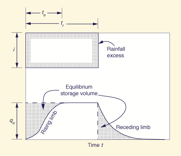
Flow over the plane can be described as follows: As excess rainfall begins, water accumulates on the plane surface and begins to flow out of the plane at its lower end. Flow at the outlet (i.e., the outflow) increases gradually from zero, while the total volume of water stored over the plane also increases gradually. Eventually, if rainfall excess continues, both outflow and total volume of water stored over the plane reach a constant value. These constants are referred to as equilibrium outflow and equilibrium storage volume. For continuing rainfall excess, outflow and storage volume remain constant and equal to the equilibrium value. Immediately after excess rainfall ceases, outflow begins to draw water from storage, gradually decreasing while depleting the storage volume. Eventually, outflow returns to zero as the storage volume is completely drained.
The process is depicted in Fig. 4-13.
The flow from start to equilibrium is called the rising limb of the overland flow hydrograph.
The flow from equilibrium back to zero is called the receding limb of the hydrograph.
The equilibrium outflow can be calculated by recognizing that at equilibrium state, the outflow must equal the inflow (i.e., rainfall excess).
Therefore,
|
i qe = ( _______ ) L 3600 | (4-19) |
in which qe = equilibrium outflow, in liters per second per meter; i = rainfall excess, in millimeters per hour; and L = plane length, in meters.
Figure 4-13 Sketch of overland flow hydrograph. |
Equation 4-19 is essentially a statement of runoff concentration, similar to Eq. 2-58 or to Eq. 4-1 with C = 1.
Whether the flow actually does concentrate and reach its equilibrium value will depend upon the duration of the rainfall excess tr relative to the time te required to reach equilibrium.
If tr > te, equilibrium is reached.
The volume of storage is the area below the line q = qe, and above the rising limb of the overland flow hydrograph, as shown in Fig. 4-13.
As a first approximation, the shaded area above the rising limb may be assumed to be equal to the area below the rising limb.
In this case, the equilibrium storage volume is:
|
qe te Se = ________ 2 | (4-20) |
in which Se = equilibrium storage volume, in liters per meter; qe = equilibrium outflow, in liters per second per meter; and te = time to equilibrium, in seconds.
In practice, surface and other irregularities cause the equilibrium state to be approached asymptotically and, therefore, the actual time to equilibrium is not clearly defined.
A value of time t corresponding to q = 0.98qe may be taken as a practical measure of te.
Then, Eq. 4-20 is only an approximation of the actual storage volume.
The equation of continuity, Eq. 4-18, can also be expressed in the following form:
|
1 ∂h u ∂h h ∂u ( ___ ) _____ + ( ____ ) _____ + ( ___ ) _____ = 1 i ∂t i ∂x i ∂x | (4-21) |
in which u = q/h = mean velocity.
The value of equilibrium outflow was obtained from Eq. 4-19 based on continuity considerations.
However, the shape of the rising and receding limbs and the time to equilibrium remain to be elucidated.
This can be obtained through the equation of momentum conservation (or equation of motion), following established principles of unsteady open channel flow [3, 9, 18].
The equation of motion, however, is a nonlinear partial differential equation.
A form of this equation with u and h as dependent variables is [18]:
|
1 ∂u u ∂h h ∂u iu ( __ ) ____ + ( __ ) ____ + ( ___ ) ____ + Sf - So + ____ = 0 i ∂ t i ∂x i ∂x gh | (4-22) |
in which Sf = friction slope, So = plane slope, g = gravitational acceleration, and all other terms have been previously defined.
All terms in Eqs. 4-21 and 4-22 are dimensionless.
The solution of Eqs. 4-21 and 4-22 can be attempted in a variety of ways.
Analytical solutions are usually based on an assumption of linearity [1, 22].
Numerical solutions have been extensively applied to stream and river flow problems [16, 18].
To date, overland flow problems have been solved with one of the following approaches:
- Storage concept,
- Kinematic wave technique,
- Diffusion wave technique, and
- Dynamic wave technique.
The storage concept is similar to that used in reservoir routing (Chapter 8).
The kinematic wave technique simulates runoff concentration in the absence of diffusion.
The diffusion wave technique simulates runoff concentration in the presence of small amounts of diffusion.
The dynamic wave technique solves the complete set of governing equations, Eqs. 4-21 and 4-22, including runoff concentration, diffusion, and dispersion (third order) processes [23].
For practical applications, the storage concept and kinematic and diffusion wave techniques can be shown to be useful approximations to the complete equations.
In principle, the kinematic wave is an improvement over the storage concept; in turn, the diffusion wave is an improvement over the kinematic wave, whereas the dynamic wave is an improvement over the diffusion wave.
Invariably, the effort involved in obtaining a solution increases in direct relation to the complexity of the equations being solved, including initial and boundary conditions.
The storage and kinematic wave techniques are described in the following sections.
A brief introduction to the diffusion wave technique is also given.
The dynamic wave solution for overland flow is outside the scope of this ebook [4].
Overland Flow Solution Based on Storage Concept
Early approaches to solve the overland flow problem are attributed to Horton [10] and Izzard [13, 14].
In particular, Horton noticed that experimental data justified a relationship between equilibrium outflow and equilibrium storage volume of the following form:
| qe = a Sem | (4-23) |
in which a and m are empirical constants.
A mean flow depth he is defined in the following way:
Se
|
he = _____ L | (4-24) |
Combining Eqs. 4-23 and 4-24:
| qe = b hem | (4-25) |
in which b = aLm, another constant.
The value of the exponent m is a function of flow regime, depending on whether the latter is laminar, turbulent (either Manning or Chezy), or mixed laminar-turbulent.
Typical values of m are shown in Table 4-3.
| ||||||||||||||||||||||||||||||||||
A conceptual estimate of time to equilibrium can be obtained by combining Eqs. 4-20 and 4-23 and solving for te:
|
2 te = ________________ qe (m -1)/m a 1/m | (4-26) |
For laminar flow conditions, b = aLm = CL, where CL is defined as follows [3]:
|
gSo CL = _________ 3 ν | (4-27) |
and ν = kinematic viscosity, a function of water temperature (see Tables A-1 and A-2, Appendix A).
The units of CL are L-1T -1.
Furthermore, with qe = iL, Eq. 4-26 reduces to the following for the case of
|
2 L 1/3 te = _____________ i 2/3 CL1/3 | (4-28) |
in which te = time to equilibrium, in seconds; L = length of overland flow plane, in meters; and
For turbulent Manning flow conditions, b = aLm = (1/n) So1/2, in which n is the Manning friction coefficient.
With qe = iL, Eq. 4-26 reduces to the following for the case of mixed laminar-turbulent flow (5/3 < m < 3):
|
2 (nL) 1/m te = ___________________ i (m - 1)/m So 1/(2m) | (4-29) |
with the same units as Eq. 4-28 (te in seconds, L in meters, i in meters per second).
As expected, time to equilibrium increases with bottom friction and plane length, and decreases with effective rainfall intensity and plane slope.
Equation 4-29 was developed by assuming the Manning formula in the rating.
Therefore, it is strictly applicable only to m = 5/3.
In practice, however, this equation is also used for mixed laminar-turbulent flow (5/3 < m < 3).
In addition, the very shallow depths that usually prevail in overland flow calculations result in a substantial increase in friction.
These differences are accounted for by using an effective roughness parameter N in lieu of the Manning friction coefficient [11].
Typical values of N are given in Table 4-4.
| ||||||||||||||||||||||||||||||||||
Rising limb of the overland flow hydrograph
The Horton-Izzard solution to the overland flow problem is based on the assumption that Eq. 4-23 is valid not only at equilibrium but also at any other time:
| q = a S m | (4-30) |
in which q = outflow at time t, and S = storage volume at time t.
This assumption is convenient because it allows an analytical solution for the shape of the overland flow hydrograph.
Equation 4-30 is the formula for a nonlinear reservoir, i.e., a function relating outflow and storage volume in a nonlinear way (m ≠ 1).
Therefore, a nonlinear reservoir is being used to model the equation of motion, Eq. 4-22.
In essence, a deterministic model (Eq. 4-22) has been replaced by a conceptual model (Eq. 4-30).
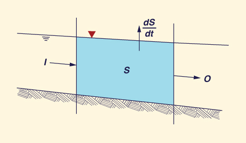
Equation 4-16 can be expressed in one space increment Δx to yield:
|
dS I - O = _____ dt | (4-31) |
in which I = inflow to the control volume, O = outflow from the control volume, and dS/dt = rate of change of storage in control volume (Fig. 4-14).
For the overland flow case, I = iL and
Therefore:
|
dS iL - q = _____ dt | (4-32) |
which through Eqs. 4-19, 4-23, and 4-30 leads to:
|
dS a Sem - a S m = ______ dt | (4-33) |
Figure 4-14 Inflow, outflow, and rate of change of storage in a control volume. |
Integrating Eq. 4-33:
|
1 1 t = ____ ∫ ____________ dS a Se m - S m | (4-34) |
and, through additional algebraic manipulation [1]:
|
1 1 t = _________________ ∫ ________________ d ( q /qe ) 1/m a 1/m qe (m - 1)/m 1 - ( q /qe ) | (4-35) |
Using Eq. 4-26, Eq. 4-35 reduces to:
|
t 1 1 ____ = ___ ∫ ______________ d ( q /qe ) 1/m te 2 1 - ( q /qe ) | (4-36) |
For m = 2, which describes a flow regime that is 75% turbulent (between laminar, for which m = 3, and 100% turbulent Manning, for which m = 5/3), the solution of Eq. 4-36 is:
|
t 1 1 + ( q /qe )1/2 ____ = ___ ln [ ___________________ ] te 4 1 - ( q /qe )1/2 | (4-37) |
which was expressed by Horton with time as independent variable as follows [1]:
|
q t ____ = tanh 2 [ 2 ( ____ ) ] qe te | (4-38) |
For m = 3 (laminar flow), the solution of Eq. 4-36 is [24]:
|
t 1 1 + (q/qe)1/3 + (q/qe)2/3 ___ = ____ ln { __________________________ } te 12 [ (q/qe)1/3 -1 ] 2 |
|
1 π 1 - ______ { ____ + arctan { - _____ [ 1 + 2 (q / qe)1/3 ] } } 2√3 6 √3 | (4-39) |
With the aid of Eq. 4-38, and Eq. 4-19 for qe and Eq. 4-29 for te, the rising limb of the overland flow hydrograph for m = 2 can be calculated.
Likewise, with the aid of
Receding limb
For m > 1, the receding limb of the overland flow hydrograph can be calculated by the following formula [24]:
|
t 1 _____ = ____________ [ (q /qe ) (1 - m )/m - 1 ] te 2 (m - 1) | (4-40) |
where q /qe = 1 for t /te = 0, i.e., the outflow is at equilibrium at the start of the recession.
Likewise, for m = 1, the hydrograph recession is as follows [24]:
|
t 1 _____ = _____ ln (q /qe ) te 2 | (4-41) |
where q /qe = 1 for t /te = 0.
Limitations
Several assumptions limit the applicability of the Horton-Izzard solution.
The most important one is the nonlinear form of the storage equation, Eqs. 4-23 and 4-30.
Izzard has suggested that the method should be restricted to cases where the product of rainfall intensity (in millimeters per hour) and plane length (in meters) (iL) does not exceed 3000.
Notwithstanding the apparent limitations, the Horton-Izzard solution of overland flow has been extensively used in the past, particularly in the design of airport drainage [3, 7].
Overland Flow Solution Based on Kinematic Wave Theory
According to this theory, Eq. 4-22 can be approximated by a single-valued flow-depth rating at any point, leading to:
| q = b h m | (4-42) |
in which b and m are constants analogous to those of Eq. 4-25.
Unlike Horton's approach, which bases the rating on the storage volume on the entire plane (Eqs. 4-23 and 4-30), the kinematic wave approach bases the rating on flow depths at individual cross sections.
This difference has substantial implications for computer modeling because whereas the Horton approach is lumped in space, the kinematic approach is not, and therefore it is better suited to distributed computation.
Reservoirs and channels
The difference between a rating based on storage volume and one based on flow depth merits further discussion. There are two distinct features in free surface flow in natural catchments:
- Reservoirs, and
- Channels.
In an ideal reservoir, the water surface slope is zero [Fig. 4-15 (a)], and, therefore, outflow and storage volume are uniquely related. If an outflow rating is desired, storage volume can be uniquely related to stage; consequently, outflow can be uniquely related to stage and flow depth. On the other hand, in an ideal channel, the water surface slope is nonzero [Fig. 4-15 (b)], and, in general, storage is a nonunique function of inflow and outflow. If a flow rating is desired, the only practical way of obtaining it is to relate flow to its depth.
Figure 4-15 (a) Ideal reservoir; (b) ideal channel. |

In the Horton approach, outflow is related to storage volume and, by extension, to the mean flow depth on the overland plane.
In contrast, in the kinematic wave approach, outflow is related to the outflow depth.
Since the typical overland flow problem has a nonzero water surface slope, it is more likely to behave as a channel rather than a reservoir.
Therefore, it would appear that the kinematic wave approach is a better model of the physical process than the storage concept.
Further analysis has shown, however, that while the kinematic wave lacks diffusion, the storage concept does not.
In this sense, the storage concept may well be a better model than the kinematic wave approach for cases featuring significant amounts of runoff diffusion.
The kinematic wave assumption, Eq. 4-42, amounts to substituting a uniform flow formula (such as Manning's) for the equation of motion, Eq. 4-22.
In essence, it says that as far as momentum is concerned, the flow is steady.
The unsteadiness of the phenomena, however, is preserved through the continuity equation, Eq. 4-18, or Eq. 4-21.
The implication of the kinematic wave assumption is that unsteady flow may be visualized as a succession of steady uniform flows, with the water surface slope remaining constant at all times.
This, of course, can be reconciled with reality only if the flow unsteadiness is very mild; that is, if the changes in stage occur very gradually.
In practice, a necessary condition for the applicability of Eq. 4-42 to unsteady flows is that the changes in momentum be negligible compared to the force driving the steady flow, i.e., gravity (the plane or channel slope).
The kinematic flow number used in overland flow applications (Eq. 4-56) serves as a quantitative measure of how kinematic a given unsteady flow condition is; that is, of the extent to which Eq. 4-42 a good surrogate of Eq. 4-22 and, therefore, a valid description of the unsteady flow phenomena.
Kinematic wave solution
The application of kinematic wave theory to the overland flow problem begins with Eq. 4-18, repeated here for convenience:
∂q ∂h
| ____ + ____ =
i ∂x ∂t | (4-18) |
Differentiating Eq. 4-42 with respect to flow depth, assuming that b and m are constants (a wide channel of constant friction) gives:
|
∂q q ____ = mbh m - 1 = m ( ____ ) = mu = c ∂h h | (4-43) |
in which c = celerity of a kinematic wave.
Since in overland flow m > 1 (Table 4-3), the celerity of a kinematic wave is greater than the mean flow velocity.
Multiplying Eqs. 4-18 and 4-43 and using the chain rule,
|
∂q ∂q ____ + c ____ = ci ∂t ∂x | (4-44) |
which is a form of the kinematic wave equation with q as the dependent variable.
Using the same approach, an expression for kinematic flow in terms of flow depth can be derived:
|
∂h ∂h ____ + c ____ = i ∂t ∂x | (4-45) |
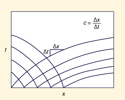
With c = dx/dt, i.e., the slope of the characteristic lines on an x-t plane (Fig. 4-16),
the left side of
Therefore:
|
dq ____ = ci dt | (4-46) |
|
dq ____ = i dx | (4-47) |
|
dh ____ = i dt | (4-48) |
|
dh i ____ = ____ dx c | (4-49) |
Figure 4-16 Characteristic lines on the x-t plane. |
In particular, Eq. 4-48 can be integrated to yield:
| h = i t | (4-50) |
which implies that the flow depth at any point along the plane increases linearly with time, provided that rainfall excess i remains constant.
The overland flow solution under the kinematic wave assumption resembles that of the storage concept, with a rising limb, an equilibrium state, and a receding limb.
Although the equilibrium flow is the same (qe = i L), the time to equilibrium is notably different, as is the shape of rising and receding limbs.
To derive the kinematic wave solution, Eq. 4-42 is expressed in terms of equilibrium outflow:
| qe = b hem | (4-51) |
in which, unlike in Eqs. 4-24 and 4-25, he is now interpreted as the equilibrium flow depth at the catchment outlet.
Dividing Eq. 4-42 by Eq. 4-50 leads to:
|
q h m ___ = ( ___ ) qe he | (4-52) |
Since h = it (Eq. 4-50), this leads to:
|
q t m ___ = ( ___ ) qe tk | (4-53) |
in which tk = kinematic time parameter, defined as:
|
he tk = _____ i | (4-54) |
Equation 4-53 is applicable for t ≤ tk.
Otherwise, the flow would exceed the equilibrium value, which is clearly a physical impossibility.
Thus, the kinematic time parameter may be interpreted as a kinematic time-to-equilibrium.
With Eq. 4-51, and since qe = iL and b = (1/n) So1/2 (for turbulent Manning friction in wide channels), the kinematic time parameter may be expressed as follows:
|
(nL) 1/m tk = ___________________ i (m - 1)/m So 1/(2m) | (4-55) |
which is the same as Eq. 4-29, albeit without the factor 2.
In other words, the analytical solution to the kinematic wave equation is a parabola (Eq. 4-53), whereas the analytical solution of the storage concept is a hyperbolic trigonometric function (see, for instance, Eq. 4-38, applicable for m = 2).
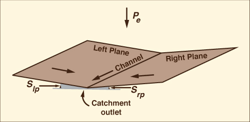
Wooding's open book
The kinematic approach to the solution of the overland flow problem was studied in detail by Iwagaki [12], Henderson and Wooding [8], Wooding [29, 30, 31], and Woolhiser and Liggett [32], among others.
Wooding developed the concept of the open book shown in Fig. 4-17, which has been extensively used in catchment modeling (Chapter 10).
The open book is formed by two overland flow planes; the outflow from the planes is lateral inflow to the channel, which conveys the flow to the catchment outlet.
Figure 4-17 Wooding's open-book catchment schematization [27]. |
Applicability of kinematic waves
Woolhiser and Liggett calculated the shape of the rising hydrograph under kinematic flow.
Furthermore, they established the limit for the applicability of the kinematic wave in terms of the kinematic flow number, defined as follows:
|
So L K = __________ F 2 ho | (4-56) |
in which K = kinematic flow number, a dimensionless number; F = Froude number corresponding to the equilibrium flow at the outlet; and ho = equilibrium flow depth at the outlet (i.e., he).
Values of K greater than 20 describe kinematic flow, while lower values do not [18].
In other words, for low K values, Eq. 4-41 is no longer a good approximation of Eq. 4-22.
In particular, since So is likely to vary within a wider range than either L, F, or ho, Eq. 4-56 could be interpreted to mean that the property of a wave being kinematic is directly related to plane slope: the steeper the slope, the greater the K value and the more kinematic the resulting flow should be.
Conversely, the milder the slope, the lower the K value and the less kinematic the flow.
The reason for this inability of the kinematic wave to account for a wide range of slopes is apparent from the nature of Eq. 4-22.
The kinematic wave accounts only for friction and plane slopes.
All other terms are excluded from the formulation and are, therefore, absent from the solution.
For very mild plane slopes, the importance of these terms may be promoted to the point where neglecting them is no longer justified.
While this appears to impose stringent limitations, the situation in practice is quite different.
Most overland flow problems have steep slopes, on the order of So = 0.01 or more, resulting in the flow being essentially kinematic, as confirmed by their kinematic flow number (Eq. 4-56).
However, much milder slopes, less than So = 0.001, result in very low kinematic flow numbers; for these cases, the kinematic wave solution may not be justified.
Kinematic shock
A source of complexity in kinematic wave solutions arises from the fact that the wave celerity in
At first, this appears to be an advantage.
Further examination, however, reveals that this property may lead to a steepening tendency of the wave.
Analytical solutions, if carried long enough (i.e., in very long channels), invariably lead to the phenomenon called kinematic shock, the steepening of the kinematic wave to the point where it attains an almost vertical face.
Kibler and Woolhiser put it in the right context when they stated [15]:
"...While the shock wave phenomenon may arise under highly selective physical circumstances, it is looked upon in this study as a property of the mathematical equations used to explore the overland flow problem rather than an observable feature of this hydrodynamic process."
In nature, small amounts of diffusion and other irregularities usually act in such a way as to control and arrest shock development.
An analytical solution, however, has no such imperfections.
In essence, the total absence of diffusion in the analytical solution permits the uncontrolled development of the kinematic shock.
Numerical solutions, however, usually have small amounts of diffusion and are, therefore, not perfect, with the shock being a rare occurrence in this case.
This fact gives rise to practical implications for stream channel and catchment routing (Chapters 9 and 10).
Comparison of storage and kinematic wave solutions
Figure 4-18 shows dimensionless rising hydrographs of storage-concept overland flow solutions for values of 1 ≤ m ≤ 3.
Note that dimensionless discharge is defined as: q* = q /qe, and dimensionless time as: t* = t /te.
For comparison, the rising hydrograph of the kinematic wave (KW) is also shown in Fig. 4-18.
This figure clearly shows that the response of the kinematic wave solution is about twice as fast as that of the storage concept (compare Eq. 4-29 for the storage concept with Eq. 4-54 for the kinematic wave).
Figure 4-18 Dimensionless rising hydrographs of overland flow using the storage concept [24]. |
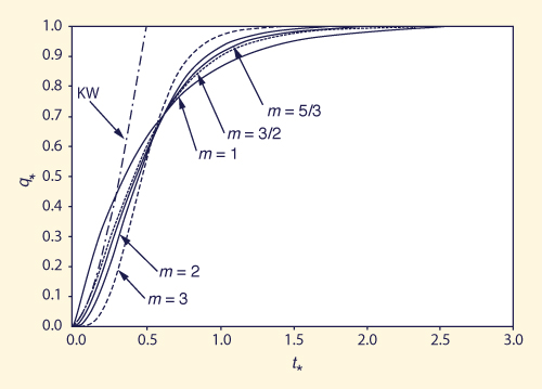
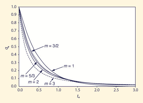
Figure 4-19 shows dimensionless receding hydrographs of storage-concept overland flow solutions for values of 1 ≤ m ≤ 3.
Figure 4-19 Dimensionless receding hydrographs of overland flow [24]. |
Overland Flow Solution Based on Diffusion Wave Theory
According to diffusion wave theory, the flow depth gradient ∂h/∂x in Eq. 4-22 is largely responsible for the diffusion mechanism, which is naturally present in unsteady free surface flows.
Therefore, its inclusion in the analysis should provide runoff concentration with diffusion.
The inclusion of the depth gradient term substantially increases the difficulty of obtaining a solution.
An established procedure is to linearize the governing equations, Eqs. 4-21 and 4-22, around reference flow values.
This entails using small-perturbation theory to develop linear analogs of these equations.
This procedure, while heuristic, has worked well in a number of applications.
Following Lighthill and Whitham [17], the linear analogs of Eqs. 4-21 and 4-22, neglecting the inertia terms (the first two terms of Eq. 4-22) and the momentum source term for simplicity, are, respectively,
|
∂h ∂h ∂u ___ + uo ___ + ho ___ = i ∂t ∂x ∂x | (4-57) |
|
∂h u 4 h ___ + So [ 2 (___) - (__)(___) ] = 0 ∂x uo 3 ho | (4-58) |
The coefficients of Eq 4-57 are constant, being the reference flow velocity uo and depth ho, respectively.
The second term of Eq. 4-58 represents a combined linear version of the friction slope Sf and channel slope So.
Furthermore, in Eq. 4-58 friction is described by the Manning formula.
If the Chezy formula is used, the factor 4/3 is replaced by 1.
Differentiating Eq. 4-58 with respect to space and eliminating the term ∂u/∂x from the resulting equation (with the aid of Eq. 4-57), the following is obtained:
|
∂h 5 ∂h uo ho ∂ 2h ___ + (___) uo ____ = i + (________) ______ ∂t 3 ∂x 2So ∂x 2 | (4-59) |
A similar expression with discharge as dependent variable may also be derived, albeit at the cost of increased algebraic manipulation (Chapter 9).
Unlike the kinematic wave equation (Eq. 4-44), which has no second-order term, the diffusion wave equation (Eq. 4-59) has a second-order term.
Therefore, the latter can describe not only runoff concentration but also diffusion.
Equation 4-59 can be expressed in the following form:
|
∂h ∂h ∂ 2h ___ + c ___ = i + νh ______ ∂t ∂x ∂x 2 | (4-60) |
in which
| c = (5/3) uo | (4-61) |
is the celerity of a diffusion wave, for turbulent Manning friction in hydraulically wide channels (overland flow), and
|
uo ho νh = ________ 2So | (4-62) |
is the hydraulic diffusivity, or channel diffusivity.
Equation 4-59 implies that the diffusion component (second-order term) is small compared with the concentration component (first-order terms) and that the channel diffusivity controls the diffusion contribution to the flow.
In effect, for very low values of So, channel diffusivity is very large.
In the limit, as channel slope approaches zero, channel diffusivity grows unbounded and Eq. 4-59 is no longer applicable.
However, for realistic mild slopes (approximately in the range 0.001-0.0001), the contribution of the diffusion term can be quite significant.
Diffusion wave theory, then, applies for the milder slopes for which kinematic wave theory is not sufficient.
Its application to catchment routing and hydrologic models of overland flow is discussed in Chapter 10.
In summary, overland flow techniques can provide more detail than the rational method in describing the peak and timing of outflow hydrographs from small catchments.
The increase in detail, however, is invariably associated with greater complexity.
In practice, it is reckoned that rainfall and abstraction modules must be coupled with the overland flow module in order to arrive at a meaningful model.
Ideally, these modules should be as detailed as the overland flow module.
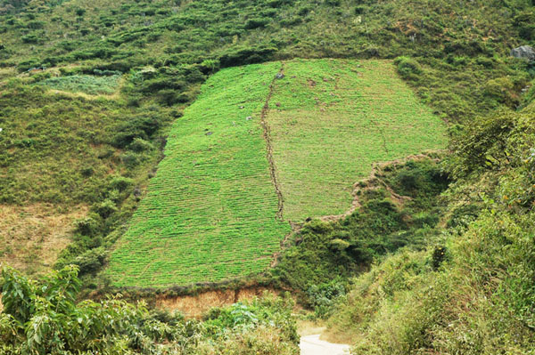
However, due to the complex spatial and temporal variability of rainfall and hydrologic abstractions, this consistency between model components is not always possible (Fig. 4-20).
Figure 4-20 Rural watershed showing the spatial variability of infiltration. |
QUESTIONS
|
|
Name three properties that characterize a small catchment. Explain each one of them.
What hydrologic processes does the rational method account for? Explain how they affect runoff.
What processes are not considered in the rational method? Explain.
How are the frequencies of storms and floods related? How does the rational method account for this difference?
What processes are included in the runoff coefficient?
Under what assumption does the rational method provide the shape of the outflow hydrograph?
Describe the phenomenon of overland flow. Contrast overland flow analysis with the rational method approach.
What crucial assumption makes the storage solution of overland flow different from the kinematic wave solution?
Why is overland flow likely to be of mixed laminar-turbulent nature? How is this modeled in practice?
What is the difference between the time of concentation (or time to equilibrium) in storage-concept and kinematic-wave overland flow models?
What is an ideal reservoir? An ideal channel? Contrast these two concepts.
What is the kinematic wave celerity? Why is it generally greater than the flow velocity?
What is the kinematic flow number? What does it describe? For what kind of channel slope is it likely that the kinematic wave solution would not be applicable?
What is kinematic shock? Why does it often occur in analytic kinematic wave solutions while it is seldom present in numerical solutions?
Contrast kinematic and diffusion wave approaches to overland flow.
Why does Eq. 4-59 describe runoff diffusion, while Eq. 4-43 does not?
What is hydraulic diffusivity?
PROBLEMS
|
|
Rain falls on a 150-ha catchment with intensity 2 cm/h and duration 2 h. Use the rational method to calculate the peak runoff, assuming runoff coefficient C = 0.6 and time of concentration
tc = 1.5 h. Rain falls on a 300-ac watershed with intensity 0.5 in./h and duration 2 h. Use the rational method to calculate the peak runoff, assuming runoff coefficient C = 0.4 and time of concentration tc = 2 h.
Rain falls on a 545-ha catchment with intensity 45 mm/h and duration 1 h. Use the rational method to calculate the peak runoff for the following conditions:
- Natural, with time of concentration 2 h and C = 0.4;
- Improved, partially paved area, with time of concentration tc = 1 h and C = 0.7.
State any assumptions used.
Rain falls on a 1.5-km2 watershed with intensity 20 mm/h and duration 2 h. Use the rational method to calculate the peak runoff for the following two conditions:
- Vegetated (natural) watershed with time of concentration tc = 3 h and C = 0.3; and
- Improved, partially paved area with time of concentration tc = 2 h and C = 0.6.
State any assumptions used.
Rain falls on a catchment with intensity 35 mm/h and duration 2 h. The catchment area is 250 ha, with time of concentration tc = 2 hand φ = 15 mm/h. Calculate the peak runoff. State any assumptions used.
Rain falls on a watershed with intensity 1 in./h and duration 3 h. The watershed area is 500 ac, with time of concentration tc = 2 h and φ = 0.3 in./h. Calculate the peak runoff. State any assumptions used.
Rain falls on a watershed with intensity 30 mm/h and duration 1 h. The watershed area is 0.8 km2 with time of concentration tc = 2 h and φ = 15 mm/h. Use the rational method to calculate the peak runoff. State any assumptions used.
Rain falls on a 125-ha catchment with the following characteristics:
- 20%, C = 0.3;
- 30%, C = 0.4;
- 50%, C = 0.6.
Calculate the peak runoff due to a storm of 45 mm/h intensity lasting 1 h. Assume time of concentration tc = 30 min.
Rain falls on a 90-ha catchment with the following characteristics:
- 12 ha, C = 0.3;
- 48 ha, C = 0.7;
- 30 ha, C = 0.9.
Calculate the peak runoff from a 50 mm/h storm lasting 2 h. Assume time of concentration tc = 2 h.
Rain falls on a 300-ha composite catchment which drains two subareas, as follows:
- Subarea A, steep, draining 20%, with time of concentration 10 min and C = 0.8; and
- Subarea B, milder steep, draining 80%, with time of concentration 60 min and C= 0.4.
Calculate the peak runoff corresponding to the 25-y-frequency. Use the following IDF function:
800T 0.2
I = ______________
(tr + 15) 0.7in which I = rainfall intensity in millimeters per hour, T = return period in years, and tr = rainfall duration in minutes. Assume linear flow concentration at the catchment outlet.
- Rain falls on a 150-ha composite catchment, which drains two subareas, as follows:
- Subarea A, steep, draining 30%, with time of concentration 20 min; and
- Subarea B, milder steep, draining 70%, with time of concentration 60 min.
The hydrologic abstraction is given in terms of φ = 25 mm/h. Calculate the 100-y-frequency peak flow. Use the following IDF function:
650T 0.22
I = _______________
(tr + 18) 0.75in which I = rainfall intensity in millimeters per hour, T = return period in years, and tr = rainfall duration in minutes. Assume linear flow concentration at the catchment outlet. State any other assumptions used.
Rain falls on a composite catchment, which drains two subareas, as follows:
- Subarea A, draining 84 ha, C = 0.4, time of concentration 30 min;
- Subarea B, draining 180 ha, C = 0.6, time of concentration 60 min.
The runoff concentration for subarea B is a nonlinear function expressed as follows:
% of time
of concentration0 10 20 30 40 50 60 70 80 90 100 % of maximum
discharge0 5 10 20 30 50 70 80 90 95 100 Calculate the 50-yr-frequency peak flow. Use the following IDF function:
52T 0.24
I = ______________
(tr + 22) 0.8in which I = rainfall intensity in millimeters per hour, T = return period in years, and tr = rainfall duration in minutes.
A developed catchment is divided into five subareas, as sketched in Fig. 4-10, with the following data:
Collection Point Subarea Increment
(ha)Travel Time
(min)C A 25 10 0.6 B 40 15 0.6 C 60 20 0.5 D 50 25 0.5 E 25 20 0.4 Calculate the 10-y-frequency peak flow. Use the following IDF function:
500T 0.18
I = _______________
(tr + 20) 0.78in which I = rainfall intensity in millimeters per hour, T = return period in years, and tr = rainfall duration in minutes.
A developed catchment is divided into five subareas, as sketched in Fig. 4-10, with the following data:
Collection Point Subarea Increment
(ha)Travel Time
(min)C A 15 5 0.7 B 30 10 0.6 C 20 15 0.4 D 10 15 0.7 E 15 15 0.9 Calculate the 10-y-frequency peak flow. Use the following IDF function:
750T 0.2
I = ______________
( tr + 25) 0.7in which I = rainfall intensity in millimeters per hour, T = return period in years, and tr = rainfall duration in minutes.
The length of an overland flow plane is L = 90 m. Determine the equilibrium outflow corresponding to a rainfall excess i = 35 mm/h.
An overland flow plane is 100 m long and 200 m wide, with time to equilibrium equal to 1 h. Estimate the equilibrium storage volume (in cubic meters) for a rainfall excess i = 54 mm/h.
Use the storage concept to calculate the time to equilibrium for an overland flow plane with the following characteristics: 100% laminar flow, plane length L = 75 m, plane slope So = 0.01, rainfall excess i = 72 mm/h, water temperature 20°C.
Calculate the mean overland flow depth (at equilibrium) under a laminar flow regime for a plane length L = 80 m, rainfall excess i = 30 mm/h, and plane slope So = 0.012. Use water temperature T = 15°C. What would be the mean overland flow depth if the water temperature increased to 25°C?
Use the storage concept to calculate the time to equilibrium for an overland flow plane with the following characteristics: turbulent Manning friction with n = 0.06, plane length L = 50 m, plane slope So = 0.02, rainfall excess i = 72 mm/h.
Calculate the rising limb of an overland flow hydrograph using Horton's equation (Eq. 4-37) assuming 75% turbulent flow. Use: Manning n = 0.06, plane length L = 60 m, plane slope So = 0.015, rainfall excess i = 30 mm/h.
Calculate the rising limb of an overland flow hydrograph using Izzard's equation (Eq. 4-39). Use: L = 60 m, So = 0.015, i = 30 mm/h, and ν = 1 cs.
Prove that Eqs. 4-37 and 4-38 are equivalent.
Calculate the receding limb of an overland flow hydrograph, using m = 3, L = 50 m, So = 0.02, i = 33 mm/h, and ν = 1 cs.
Derive the formula for the kinematic time parameter for 100% laminar flow (m = 3).
Using the formula derived in Problem 4-24, calculate the rising limb of an overland flow hydrograph using the kinematic wave approach, assuming plane length L = 100 m, plane slope So = 0.01 , rainfall excess i = 25 mm/ h, and water temperature T = 20°C.
An overland flow plane has the following characteristics: plane length L = 35 m, plane slope So = 0.008, Manning n = 0.08, rainfall excess i = 55 mm/ h. Determine if the kinematic wave approximation is applicable to this set of overland flow conditions.
Calculate the hydraulic (channel) diffusivity for each of the following two flow conditions:
Bed slope So = 0.005, mean flow depth ho = 0.01 m. and mean velocity uo = 0.05 m/ s; and
Bed slope So = 0.00005, mean flow depth ho = 0.02 m, and mean velocity uo = 0.1 m/ s.
REFERENCES
|
|
Agricultural Research Service. U.S. Department of Agriculture. (1973). "Linear Theory of Hydrologic Systems," Technical Bulletin No. 1468, (J. C. 1. Dooge, author). Washington, D.C.
American Society of Civil Engineers. (1960). "Design and Construction of Sanitary and Storm Sewers," Manual of Engineering Practice No. 37, also Water Pollution Control Federation Manual of Practice No. 9.
Chow, V. T. (1959). Open Channel Hydraulics. New York: McGraw-Hill.
Chow, V. T., and A. Ben-Zvi. (1973). "Hydrodynamic Modeling of Two-dimensional Watershed Flow," Journal of the Hydraulics Division, ASCE, Vol. 99, No. HYll, Nov. pp. 2023-2040.
County of Kern, California. (1985). "Revision of Coefficient of Runoff Charts," Office Memo, dated January 18, 1985.
County of Solano, California. (1977). "Hydrology and Drainage Design Procedure," prepared by Water Resources Engineers, Inc., Walnut Creek, California, October.
Hathaway, G. A. (1945). "Design of Drainage Facilities," in Military Airfields, A Symposium, Transactions, American Society of Civil Engineers. Vol. 110, pp. 697-733.
Henderson, F. M., and R. A. Wooding. (1964). "Overland Flow and Groundwater Flow from a Steady Rainfali of Finite Duration," Journal of Geophysical Research. Vol. 69, No.8, April, pp. 1531-1540.
Henderson, F. M. (1965). Open Channel Flow. New York: MacMillan.
Horton, R. E. (1938). "The Interpretation and Application of Runoff Plot Experiments with Reference to Soil Erosion Problems," Proceedings, Soil Science Society of America. Vol. 3, pp. 340-349.
Hydrologic Engineering Center, U.S. Army Corps of Engineers. (1998). "HEC-1, Flood Hydrograph Package, Users Manual," September 1981, revised January 1985, revised 1998.
Iwagaki, Y. (1955). "Fundamental Studies on the Runoff Analysis by Characteristics," Bulletin, Disaster Prevention Research Institute, Vol. 10, Kyoto University, December.
Izzard, C. F. (1944). "The Surface Profile of Overland Flow," Transactions. American Geophysical Union, Vol. 25, No.6, pp. 959-968.
Izzard, C. F. (1946). "Hydraulics of Runoff from Developed Surfaces," Proceedings. Highway Research Board, Washington, D.C., Vol. 26, pp. 129-146.
Kibler, D. F., and D. A. Woolhiser. (1970). "The kinematic cascade as a hydrologic model," Hydrology Paper No. 39, Colorado State University, Fort Collins, Colo., March.
Lai, C. (1986). "Numerical Modeling of Unsteady Qpen Channel Flow," in Advances in Hydroscience. Vol. 14. Orlando: Academic Press.
Lighthill. M. H., and G. B. Whitham. (1955). "On Kinematic Waves. 1. Flood Movement in Long Rivers," Proceedings, Royal Society. London, Vol. A229, May, pp. 281-316.
Mahmood, K., and Yevjevich, V. (1975). Unsteady Flow in Open Channels, in 3 volumes. Fort Collins, Colo.: Water Resources Publications.
Miller, W. A., and Cunge, J. A. (1975). "Simplified Equations of Unsteady Flow," in Unsteady Flow in Open Channels, K. Mahmood and V. Yevjevich, eds. , Fort Collins, Colo. : Water Resources Publications.
NOAA National Weather Service. (1973). Atlas 2: Precipitation Atlas of the Western United States.
NOAA National Weather Service. (1977). "Five- to 60-Minute Precipitation Frequency for the Eastern and Central United States," Technical Memorandum NWS HYDRO-35.
Ponce, V. M., and D. B. Simons. (1977). "Shallow Wave Propagation in Open Channel Flow," Journal of the Hydraulics Division, ASCE, Vol. 103, No. HY12, December, pp. 1461-1476.
Ponce, V. M. (1994). "New perspective on the convection-diffusion-dispersion equation," Water Resources Research, Vol. 30, No. 5, May, pp. 1619-1620.
Ponce, V. M., O. I. Cordero-Braña, and S. Y. Hasenin. (1997). "Generalized conceptual modeling of dimensionless overland flow hydrographs," Journal of Hydrology, 200, pp. 222-227.
Rantz, S. E. (1971). "Suggested Criteria for Hydrologic Design of Storm-drainage Facilities in the San Francisco Bay Region, California," U. S. Geological Survey Open-file Report, Menlo Park, California.
San Diego County. (1985). Hydrology Manual, San Diego, California, revised January.
Schaake, Jr., J. C., Geyer, and 1. W. Knapp. (1967). "Experimental Examination of the 'Rational Method," Journal of the Hydraulics Division, ASCE, Vol. 93, No. HY6, November, pp. 353-370.
Weather Bureau, U.S. Dept. of Commerce. (1963). "Rainfall Frequency Atlas of the United States for Durations from 30 Minutes to 24 Hours and Return Periods from 1 to 100 Years," Technical Paper No. 40.
Wooding, R. A. (1965) "A Hydraulic Model for the Catchment-stream Problem, I. Kinematic Wave Theory," Journal of Hydrology, Vol. 3, Nos. 3/4, pp. 254-267.
Wooding, R. A. (1965) "A Hydraulic Model for the Catchment-stream Problem, II. Numerical Solutions," Journal of Hydrology, Vol. 3, Nos. 3/4, pp. 268-282.
Wooding, R. A. (1965) "A Hydraulic Model for the Catchment-stream Problem, III. Comparison with Runoff Observations," Journal of Hydrology, Vol. 4, pp. 21-37.
Woolhiser, D. A., and Liggett, J. A. (1967). "Unsteady One-dimensional Flow Over a Plane: The Rising Hydrograph," Water Resources Research, Vol. 3, pp. 753-771.
| http://engineeringhydrology.sdsu.edu |
|
150713 |