|
|
|
CHAPTER 2: HYDROLOGIC PRINCIPLES |
|
"Discharge by wells must be balanced by an increase in the recharge of the aquifer, or by a decrease in the old natural discharge, or by a loss of storage, or by a combination of these." Charles V. Theis (1940) |
|
This chapter is divided into four sections. Section 2.1 deals with precipitation, its meteorological aspects, quantitative description, spatial and temporal variations, and data sources. Section 2.2 discusses hydrologic abstractions that are important in engineering hydrology: interception, infiltration, surface storage, evaporation, and evapotranspiration. Section 2.3 defines geometric and other catchment properties relevant to hydrologic analysis. Section 2.4 deals with runoff analysis, both in a qualitative and quantitative way. The concepts presented in this chapter are of an introductory nature, intended to provide the necessary background for the more specialized study that will follow. |
2.1 PRECIPITATION
|
|
Introduction
Engineering hydrology takes a quantitative view of the hydrologic cycle. Generally, equations are used to describe the interaction between the various phases of the hydrologic cycle. As shown in Chapter 1, the following basic equation relates precipitation and surface runoff:
| Q = P - L | (2-1) |
in which Q = surface runoff, P = precipitation; and L = losses, or hydrologic abstractions. The latter term is interpreted as the summation of the various precipitation-abstracting phases of the hydrologic cycle.
Rainfall is the liquid form of precipitation; snowfall and hail are the solid forms. In common usage, the word rainfall is often used to refer to precipitation. Exceptions are the cases where a distinction between liquid and solid precipitation is warranted.
Generally, the catchment has an abstractive capability that acts to reduce total rainfall into effective rainfall. The difference between total rainfall and effective rainfall is the losses or hydrologic abstractions. The abstractive capability is a characteristic of the catchment, varying with its level of stored moisture. Hydrologic abstractions include interception, infiltration, surface storage, evaporation, and evapotranspiration. The difference between total rainfall and hydrologic abstractions is called runoff. Therefore, the concepts of effective rainfall and runoff are equivalent.
The terms in Eq. 2-1 can be expressed as rates (millimeters per hour, centimeters per hour, or inches per hour), or when integrated over time, as depths (millimeters, centimeters or inches). In this sense, a given depth of rainfall or runoff is a volume of water uniformly distributed over the catchment area.
Meteorological Aspects
The earth's atmosphere contains water vapor. The amount of water vapor may be conveniently expressed in terms of a depth of precipitable water. This is the depth of water that would be realized if all the water vapor in the air column above a given area were to condense and precipitate on that area.
There is an upper limit to the amount of water vapor in an air column. This upper limit is a function of the air temperature. The air column is considered to be saturated when it contains the maximum amount of water vapor for its temperature. Lowering the air temperature results in a reduction of the air column's capacity for water vapor. Consequently, an unsaturated air column, i.e., one that has less than the maximum amount of water vapor for its temperature, can become saturated without the actual addition of moisture if its temperature is lowered to a level at which the actual amount of water vapor will produce saturation. The temperature to which air must be cooled, at constant pressure and water vapor content, to reach saturation is called the dewpoint. Condensation usually occurs at or near saturation of the air column.
Cooling of Air Masses. Air can be cooled by many processes. However, adiabatic cooling by reduction of pressure through lifting is the only natural process by which large air masses can be cooled rapidly enough to produce appreciable precipitation. The rate and amount of precipitation are a function of the rate and amount of cooling and of the rate of moisture inflow into the air mass to replace the water vapor that is being converted into precipitation.
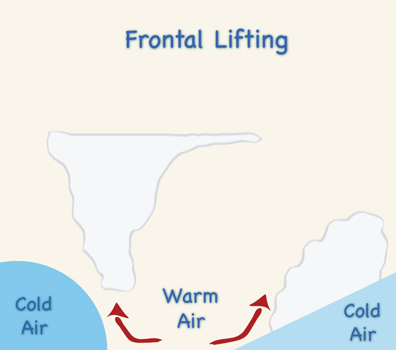
The lifting required for the rapid cooling of large air masses is due to four processes [72]:
- Frontal lifting,
- Orographic lifting,
- Lifting due to horizontal convergence, and
- Thermal lifting.
More than one of these processes is usually active in the lifting associated with the heavier precipitation rates and amounts.
Frontal lifting takes place when relatively warm air flowing towards a colder (hence denser) air mass is forced upward, with the cold air acting as a wedge (Fig. 2-1 (a)). Cold air overtaking warmer air will produce the same result by wedging the latter aloft. The surface of separation between the two different air masses is called a frontal surface. A frontal surface always slopes upward toward the colder air mass; the intersection of the frontal surface with the ground is called a front .
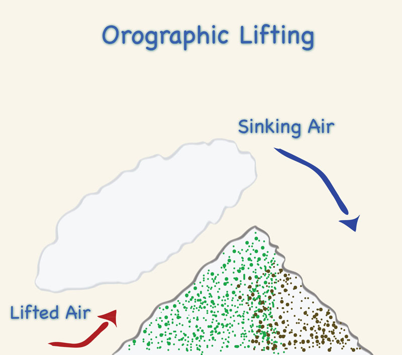
Orographic lifting occurs when air flowing toward an orographic barrier (i.e., mountain) is forced to rise in order to pass over it (Fig. 2-1 (b)). The slopes of orographic barriers are usually steeper than the steepest slopes of frontal surfaces. Consequently, air is cooled much more rapidly by orographic lifting than by frontal lifting.
|
|
|
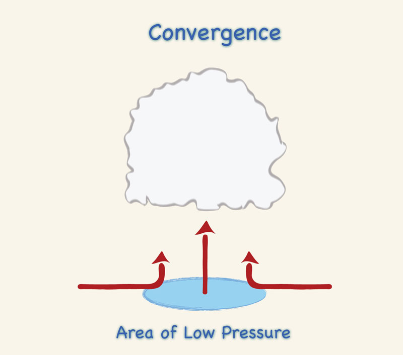
Lifting due to horizontal convergence is also important in the production of clouds and precipitation. Convergence occurs when the pressure and wind (velocity) fields act to concentrate inflow of air into a particular area, such as a low-pressure area (Fig. 2-1 (c)). If this convergence takes place in the lower layers of the atmosphere, the tendency to pile up forces the air upward, resulting in its cooling. Even when precipitation does not result from convergence alone, subsequent precipitation triggered by other processes may be more intense if convergence has occurred.
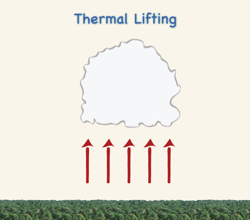
Thermal lifting is caused by local heating. As heated surface air becomes buoyant, it is forced to rise, resulting in its cooling. If the local heated air contains enough moisture and rises far enough, saturation will be reached and cumulus clouds will form (Fig. 2-1 (d)). Thermal lifting is more pronounced in the warm season. Rainfall associated with thermal lifting is likely to be scattered in geographic extent. In flat country, the greatest convective activity is over the hottest surfaces; in mountain country, it is greatest over the highest peaks and ridges.
|
|
Condensation of Water Vapor into Liquid or Solid Form. Condensation is the process by which water vapor in the atmosphere is converted into liquid droplets or, at low temperatures, into ice crystals. The results of the process are often, but not always, visible in the form of clouds, which are airborne liquid water droplets or ice crystals or a mixture of these two.
Saturation does not necessarily result in condensation. Condensation nuclei are required for the conversion of water vapor into droplets. Among the more effective condensation nuclei are certain products of combustion and salt particles from the sea. There are usually enough condensation nuclei in the air to produce condensation when the water vapor reaches saturation point.
Growth of Cloud Droplets and Ice Crystals to Precipitation Size. When air is cooled below its initial saturation, so that temperature and condensation continues to take place, liquid droplets or ice crystals tend to accumulate in the resulting cloud. The rate at which this excess liquid and solid moisture is precipitated from the cloud depends upon: (1) the speed of the upward current producing the cooling, (2) the rate of growth of the cloud droplets into raindrops heavy enough to fall through the upward current, and (3) a sufficient inflow of water vapor into the area to replace the precipitated moisture.
Water droplets in a typical cloud usually average about 0.01 mm in radius and weigh so little at an upward current of only 0.0025 m/s is sufficient to keep them from falling. Although no definite drop size can be said to mark the boundary between cloud and raindrops, a radius of 0.1 mm has been generally accepted. The radius of most raindrops reaching the ground is usually much greater than 0.1 mm and may reach 3 mm. Drops larger than this tend to break into smaller drops because the surface tension is insufficient to withstand the distortions the drop undergoes in falling through the air. Drops of 3 mm radius have a terminal velocity of about 10 m/s; therefore, an unusually strong upward current would be required to keep a drop of this size from falling.
Various theories have been advanced to explain the growth of a cloud element into a size that can precipitate. The two principal processes in the formation of precipitation are: (1) the ice crystal process, and (2) the coalescence process [29]. These two processes may operate together or separately. The ice crystal process involves the presence of ice crystals in a supercooled (cooled to below freezing) water cloud. Due to the fact that saturation vapor pressure over water is greater than that over ice, there is a vapor pressure gradient from water drops to ice crystals. This causes the ice crystals to grow at the expense of the water drops and, under favorable conditions, to attain precipitation size. The ice crystal process is operative only in supercooled water clouds, and it is most effective at about -15oC.
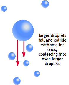
The coalescence process is based on the difference in fall velocities and consequent collisions to be expected between cloud elements of different sizes (Fig. 2-2). The rate of growth of cloud elements by coalescence depends upon the initial range of particle sizes, the size of the largest drops, the drop concentration, and the sizes of the aggregated drops. The electric field and drop charge may affect collision efficiencies and may therefore be important factors in the release of precipitation from clouds [71]. Unlike the ice crystal process, the coalescence process occurs at any temperature, lts effectiveness varying from solid to liquid particles.
Fig. 2-2 The coalescence process (cmmap.org). |
Forms of Precipitation. Precipitation occurs primarily in the form of drizzle, rain, hail, or snow (Fig. 2-3). Drizzle consists of tiny liquid water droplets, usually between 0.1 and 0.5 mm in diameter, falling at intensities rarely exceeding 1 mm/h. Rain consists of liquid water drops, mostly larger than 0.5 mm in diameter. Rainfall refers to amounts of liquid precipitation. Rainfall intensities can be classified as: light, up to 3 mm/h; moderate, from 3 to 10 mm/h; and heavy, over 10 mm/h. A rainstorm is a rainfall event lasting a clearly defined duration.
Fig. 2-3 Forms of precipitation. |
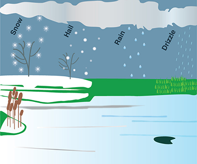
Hail is composed of solid ice stones or hailstones. Hailstones may be spheroidal, conical, or irregular in shape and may range from about 5 to over 125 mm in diameter. A hailstorm is a precipitation event in the form of hail.
Snow is composed of ice crystals, primarily in complex hexagonal form and often aggregated into snowflakes that may reach several millimeters in diameter. Snowfall is precipitation in the form of snow. A snowstorm is a snowfall event with a clearly defined duration. Snowpack is the volume of snow accumulated on the ground after one or more snowstorms. Snowmelt, or melt, is the volume of snow that has changed from solid to liquid state and is available for runoff.
Factors affecting precipitation. Table 2-1 shows the various factors affecting precipitation and their effect on: (a) moisture availability, (b) condensation, and (c) coalescence. Factors No. 1 to 7 are entirely of natural origin and, therefore, not subject to anthropogenic control. Factor No. 8 may be subject to either natural or anthropogenic control. Factor No. 9 is the only factor which is subject to anthropogenic control.
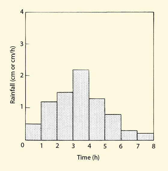
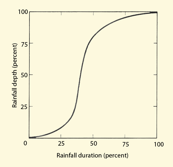
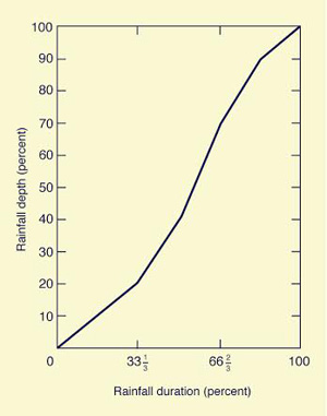
A rainfall event, or storm, describes a period of time having measurable and significant rainfall, preceded and followed by periods with no measurable rainfall. The time elapsed from start to end of the rainfall event is the rainfall duration. Typically, rainfall duration is measured in hours. However, for very small catchments it may be measured in minutes, while for very large catchments it may be measured in days. Rainfall durations of 1, 2, 3, 6, 12, and 24 h are common in hydrologic analysis and design. For small catchments, rainfall durations can be as short as 5 min. Conversely, for large river basins, durations of 2 d and longer may be applicable [78]. Rainfall depth is measured in mm, cm, or in., considered to be uniformly distributed over the catchment area. For instance, a 60-mm, 6-h rainfall event produces 60 mm of depth over a 6-h period. Rainfall depth and duration tend to vary widely, depending on geographic location, climate, microclimate, and time of the year. Other things being equal, larger rainfall depths tend to occur more infrequently than smaller rainfall depths. For design purposes, rainfall depth at a given location is related to the frequency of its occurrence. For instance, 60 mm of rainfall lasting 6 h may occur on the average once every 10 y at a certain location. However, 80 mm of rainfall lasting 6 h may occur on the average once every 25 y at the same location. Average rainfall intensity is the ratio of rainfall depth to rainfall duration. For example, a rainfall event producing 60 mm in 6 h represents an average rainfall intensity of 10 mm/h. Rainfall intensity, however, varies widely in space and time, and local or instantaneous values are likely to be very different from the spatial and temporal average. Typically, rainfall intensities are in the range 0.1-30 mm/h, but can be as large as 150 to 350 mm/h in extreme cases. Rainfall frequency refers to the average time elapsed between occurrences of two rainfall events of the same depth and duration. The actual elapsed time varies widely and can therefore be interpreted only in a statistical sense. For instance, if at a certain location a 100-mm rainfall event lasting 6 h occurs on the average once every 50 y, the 100-mm, 6-h rainfall frequency for this location would be 1 in 50 years, 1/50, or 0.02. The reciprocal of rainfall frequency is referred to as return period, or recurrence interval. In the case of the previous example, the return period corresponding to a frequency of 0.02 is 50 y. Generally, larger rainfall depths tend to be associated with longer return periods. The longer the return period, the longer the historical record needed to ascertain the statistical properties of the distribution of annual maximum rainfall. Due to the paucity of long rainfall records, extrapolations are usually necessary to estimate rainfall depths associated with long return periods. These extrapolations entail a certain measure of risk. When the risk involves human life, the concepts of rainfall frequency and return period are no longer considered adequate for design purposes. Instead, a reasonable maximization of the meteorological factors associated with extreme precipitation is used, leading to the concept of Probable Maximum Precipitation (PMP). For a given geographic location, catchment area, event duration, and time of the year, the PMP is the theoretically greatest depth of precipitation. In flood hydrology studies, the PMP is used as a basis for the calculation of the Probable Maximum Flood (PMF). For certain projects, a precipitation depth less than the PMP may be justified on economic grounds. This leads to the concept of Standard Project Storm (SPS). The SPS is taken as an appropriate percentage of the applicable PMP and is used to calculate the Standard Project Flood (SPF) (Chapter 14). Temporal and Spatial Variation of Precipitation Temporal Rainfall Distribution. Rainfall intensities for events of short duration (1 h or less) can usually be expressed as an average value, obtained by dividing rainfall depth by rainfall duration. For longer events, instantaneous values of rainfall intensity are likely to become more important, particularly for flood peak determinations. The temporal rainfall distribution depicts the variation of rainfall depth within a storm duration. It can be expressed in either discrete or continuous form. The discrete form is referred to as a hyetograph, a histogram of rainfall depth (or rainfall intensity) with time increments as abscissas and rainfall depth (or rainfall intensity) as ordinates, as shown in Fig. 2-4 (a). The continuous form is the temporal rainfall distribution, a function describing the rate of rainfall accumulation with time. Rainfall duration (abscissas) and rainfall depth (ordinates) can be expressed in percentage of total value, as shown in Fig. 2-4 (b). The dimensionless temporal rainfall distribution is used to convert a storm depth into a hyetograph, as shown in the following example.
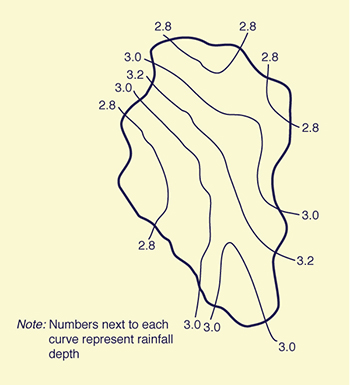
Spatial Rainfall Distribution. Rainfall varies not only temporally but also spatially, i.e., the same amount of rain does not fall uniformly over the entire catchment. Isohyets are used to depict the spatial variation of rainfall. An isohyet is a contour line showing the loci of equal rainfall depth (Fig. 2-6 (a)).
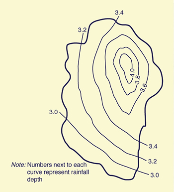
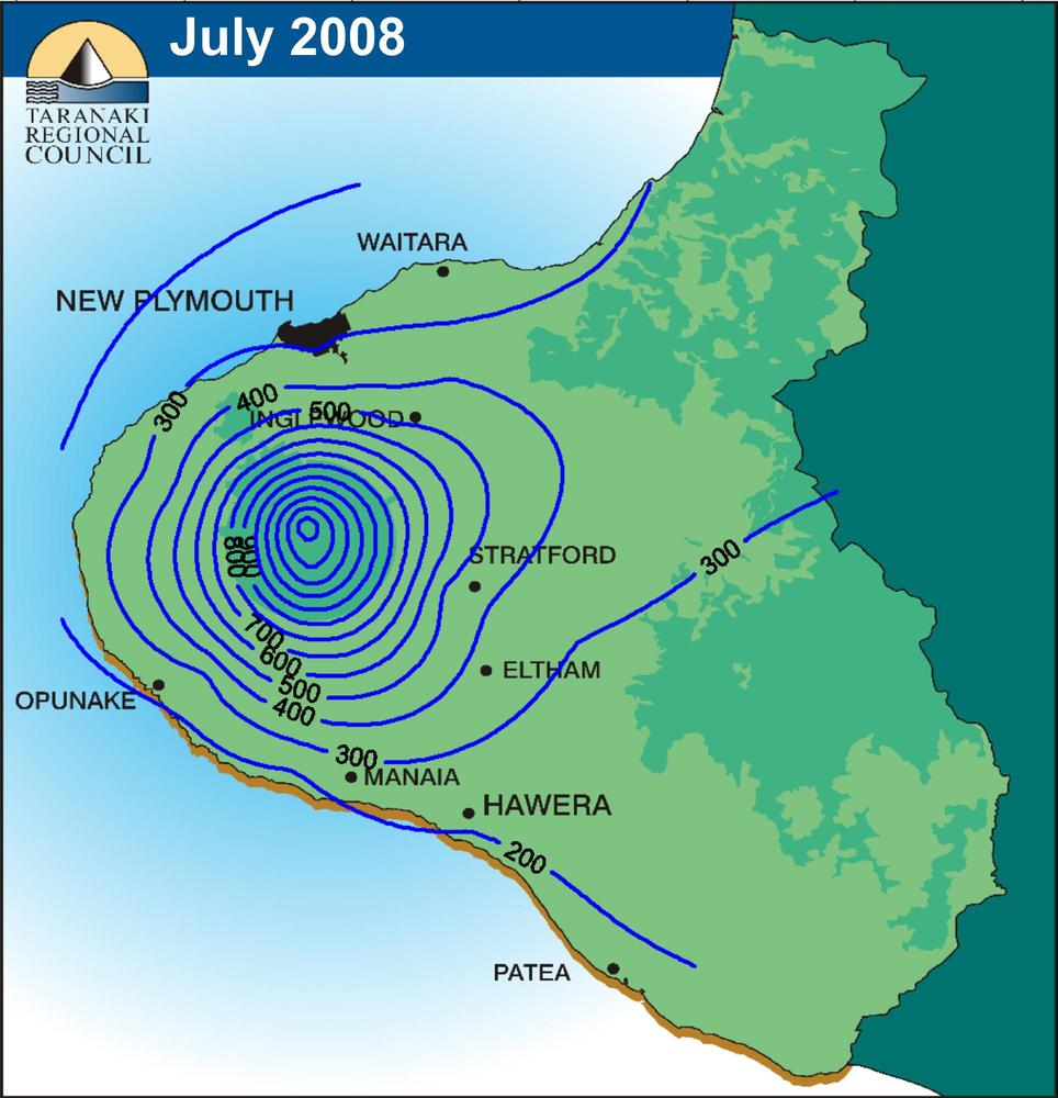
Individual storms may have a spatial distribution or pattern in the form of concentric isohyets of approximately elliptic shape. This gives rise to the term storm eye to depict the center of the storm (Fig. 2-6 (b)). In general; storm patterns are not static, moving gradually in a direction approximately parallel to that of the prevailing winds. Isohyets are also used to show spatial rainfall patterns for a given time period. Figure 2-7 shows an example of spatial rainfall distribution for the month of July 2008 in Taranaki, New Zealand.
| |||||||||||||||||||||||||||||||||||||||||||||||||||||||||||||||||||||||||||||||||||||||
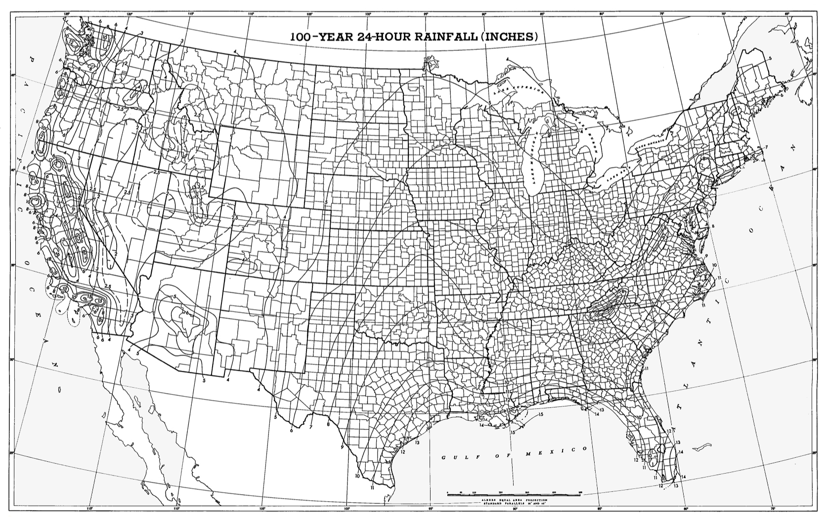
For regional rainfall mapping, isohyets are commonly referred to as isopluvials. Isopluvial maps for the United States are published by the National Weather Service [58, 59, 85-88]. These maps show contours of equal rainfall depth, applicable for a range of durations, frequencies, and geographical locations; see, for example, Fig. 2-8 for San Diego County, California, and Fig. 2-9 for the contiguous United States.
Fig. 2-8 100-yr 24-h isopluvials for San Diego County, California (0.1 in) (Source: NOAA) (Click -here- to display). |
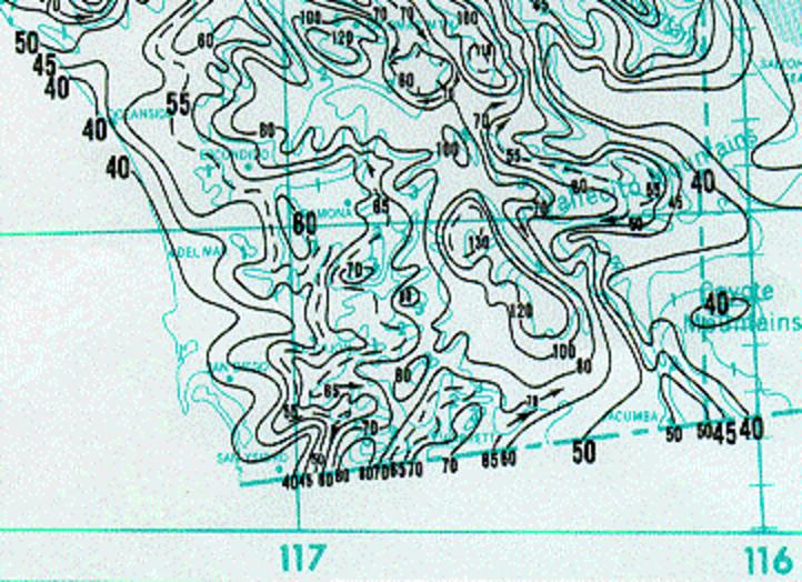
Fig. 2-9 100-yr 24-h isopluvials for the contiguous United States (in.) (NOAA) (Click -here- to display). |
For large catchments, highly intensive storms (thunderstorms) may cover only a fraction of the whole basin, yet they may lead to severe flooding in localized areas. The role of thunderstorms in determining the flood potential of large basins is usually assessed on an individual basis.
Average Precipitation Over an Area. A precipitation (or rainfall) amount is measured with rain gages. During a given storm, it is likely that the depth measured by two or more rain gages of the same type will not be the same. In hydrologic analysis, it is often necessary to determine a spatial average of the rainfall depth over the catchment. This is accomplished by either of the following methods:
- Average rainfall,
- Thiessen polygons, and
- Isohyetal curves.
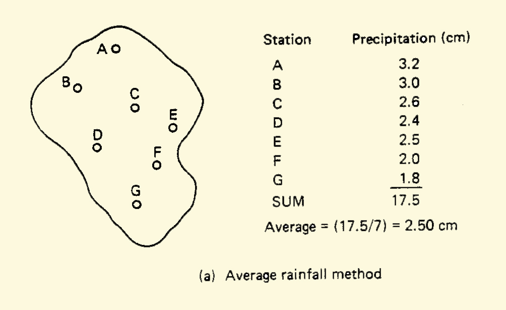
In the average rainfall method, the rainfall depths measured by the rain gages located within the catchment are tabulated. These rainfall depths are then averaged to find the average precipitation over the catchment, as shown in Fig. 2-10 (a).
Fig. 2-10 (a) Average rainfall method (Click -here- to display). |
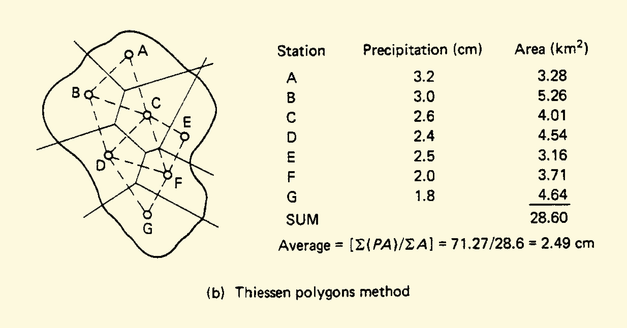
In the Thiessen polygons method, the locations of the rain gages are plotted on a scale map of the catchment and surrounding area. The locations (stations) are joined with straight lines in order to form a pattern of triangles, preferably with sides of approximately equal length. Perpendicular bisectors to the sides of these triangles are drawn to enclose each station within a polygon called a Thiessen polygon, circumscribing an area of influence, as shown in Fig. 2-10 (b). The average precipitation over the catchment is calculated by weighing each station's rainfall depth in proportion to its area of influence.
Fig. 2-10 (b) Thiessen polygons method (Click -here- to display). |
In the isohyetal method, the locations of the rain gages are plotted on a scale map of the catchment and surrounding area. Each station's rainfall depth is used to draw isohyets throughout the catchment in a manner similar to that used in the preparation of topographic contour maps. The mid-distance between two adjacent isohyets is used to delineate the area of influence of each isohyet, as shown in Fig. 2-10 (c). The average precipitation over the catchment is calculated by weighing each isohyetal increment in proportion to its area of influence.
Fig. 2-10 (c) Isohyetal method (Click -here- to display). |
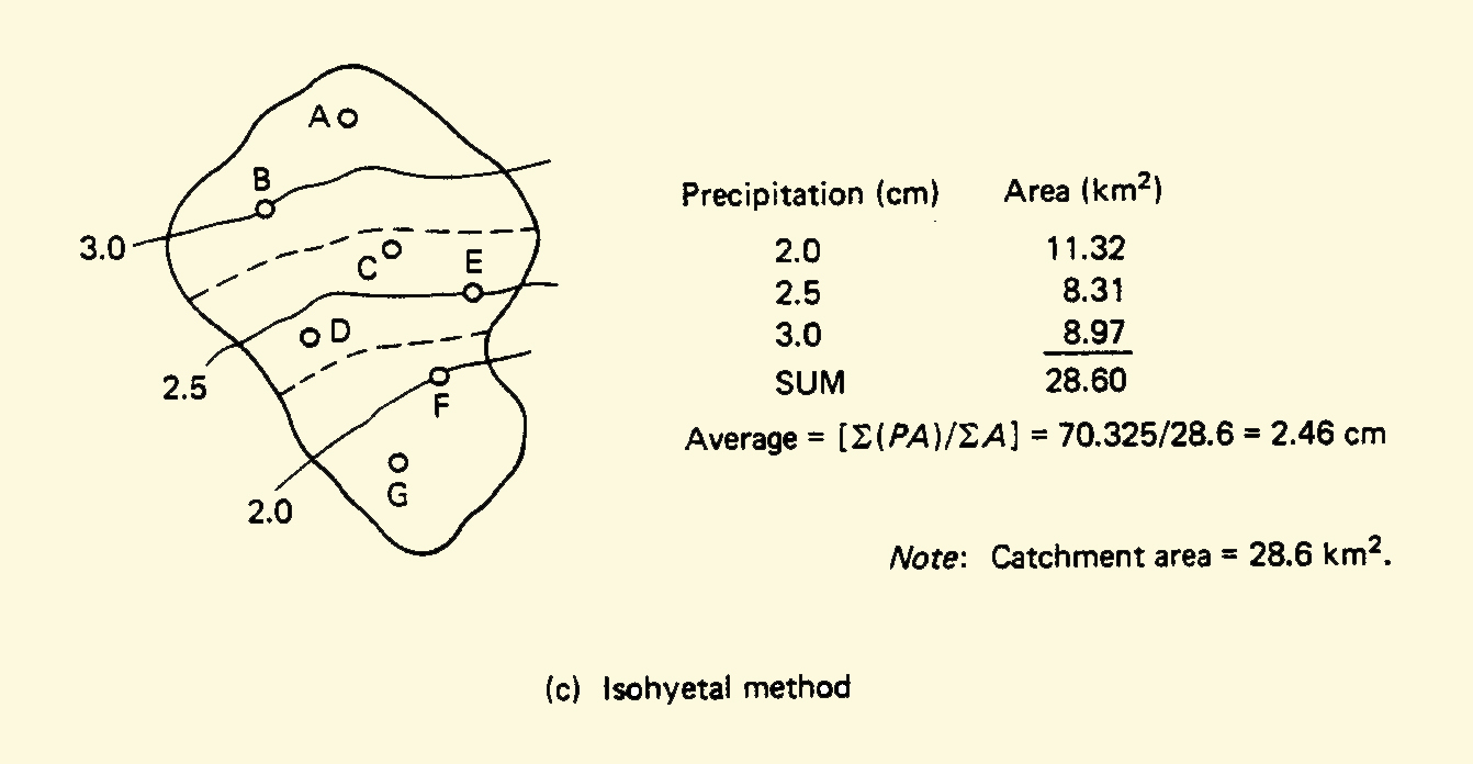
The isohyetal method is regarded as more accurate than either the Thiessen polygons or average rainfall methods. This is particularly the case when averaging precipitation over catchments where orographic effects have a significant influence on the local storm pattern. The Thiessen polygons method is generally more accurate than the average rainfall method. The increase in accuracy is likely to be more marked when averaging precipitation over catchments with widely varying rainfall depths or large differences in areas of influence.
Storm Analysis
Storm Depth and Duration. Storm depth and duration are directly related, storm depth increasing with duration. An equation relating storm depth and duration is:
| h = c t n | (2-2) |
in which h = storm depth, in centimeters; t = storm duration, in hours; c = a coefficient; and n = an exponent (a positive real number less than 1). Typically, n varies between 0.2 and 0.5, indicating that storm depth increases at a lesser rate than storm duration. By analyzing storm data on a regional or local basis, Eq. 2-2 can be used to predict storm depth as a function of storm duration. The applicability of such an equation, however, is limited to the regional or local conditions for which it was derived.
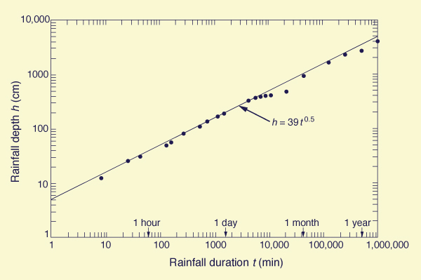
Equation 2-2 can also be used to study the characteristics of extreme rainfall events. A logarithmic plot of depth-duration data for the world's greatest observed rainfall events (Table 2-2) results in the following enveloping line:
| h = 39 t 0.5 | (2-3) |
in which h = rainfall depth, in centimeters, and t = rainfall duration, in hours. The data of Table 2-2 are plotted in Fig. 2-11, including the enveloping line, Eq. 2-3.
| ||||||||||||||||||||||||||||||||||||||||||||||||||||||||||||||||||||||||||||||||||||||||||||||||||||
Fig. 2-11 Depth-duration data for the world's greatest observed rainfall events. |
Storm Intensity and Duration. Storm intensity and duration are inversely related. From Eq. 2-2, an equation linking storm intensity and duration, can be obtained by differentiating rainfall depth with respect to duration, to yield:
|
dh ______ = i = c n t n -1 dt | (2-4) |
in which i = storm intensity. Simplifying,
|
a i = ______ t m | (2-5) |
in which a = cn, and m = 1 - n. Since n is less than 1, it follows that m is also less than 1.
Another intensity-duration model is the following:
|
a i = _________ t + b | (2-6) |
in which a and b are constants to be determined by regression analysis (Chapter 7).
A general intensity-duration model combining the features of Eqs. 2-5 and 2-6 is:
|
a i = _____________ ( t + b ) m | (2-7) |
For b = 0, Eq. 2-7 reduces to Eq. 2-5; for m = 1, Eq. 2-7 reduces to Eq. 2-6.
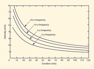
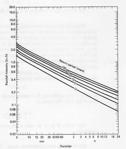
Intensity-Duration-Frequency. For small catchments it is often necessary to determine several intensity-duration curves, each for a different frequency or return period. A set of intensity-duration-frequency curves is referred to as IDF curves, with duration plotted in the abscissas, intensity in the ordinates, and frequency (or alternatively, return period) as curve parameter. Either arithmetic (Fig. 2-12 (a)) or logarithmic (Fig. 2-12 (b)) scales are used in the construction of IDF curves. Such curves are developed by government agencies for use in urban storm-drainage design and other applications (Chapter 4).
A formula for IDF curve can be obtained by assuming that the constant a in Eqs. 2-5 through 2- 7 is related to return period T as follows:
| a = k T n | (2-8) |
in which k = a coefficient; T = return period; and n = an exponent (not related to that of Eq. 2-2). This leads to
|
k T n i = _____________ ( t + b ) m | (2-9) |
The values of k, b, m, and n are evaluated from measured data or local experience.
|
|
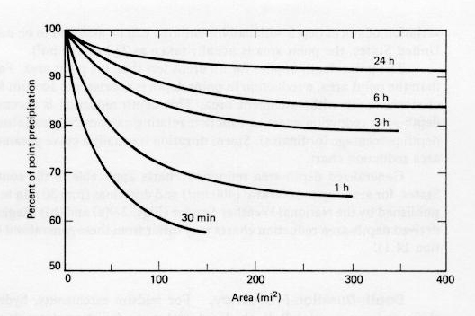
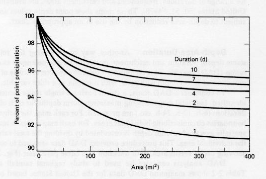
Storm Depth and Catchment Area. Generally, the greater the catchment area, the smaller the spatially averaged storm depth. This variation of storm depth with catchment area has led to the concept of point depth, defined as the storm depth associated with a given point area. A point area is the smallest area below which the variation of storm depth with catchment area can be assumed to be negligible. In the United States, the point area is usually taken as 25 km2 (10 mi2).
The point depth applies for all areas less than the point area. For areas greater than the point area, a reduction in point depth is necessary to account for the decrease of storm depth with catchment area. This depth reduction is accomplished with a depth-area reduction chart, a function relating catchment area (abscissas) to point depth percentage (ordinates). Storm duration is usually a curve parameter in a depth-area reduction chart.
Generalized depth-area reduction charts applicable to the contiguous United States, for areas up to 1000 km2 (400 mi2) and durations from 30 min to 10 d have been published by the National Weather Service (Figs. 2-13 (a) and (b)). Regional and locally derived depth-area reduction charts may differ from these generalized charts (see Section 14.1).
|
|
Depth-Duration-Frequency. For midsize catchments, hydrologic analysis shifts its focus to rainfall depth. Isopluvial maps depicting storm depths, applicable for a range of durations, frequencies and catchment areas, are available for the entire United State [58, 59, 85-88]. These maps show point depth values and are therefore subject to depth-area reduction by the use of an appropriate chart.
Depth-Area-Duration. Another way of describing the relation between storm depth, duration and catchment area is the technique known as depth-area-duration (DAD) analysis. This technique is basically an alternate way of portraying the reduction of storm depth with area, with duration as a third variable.
To construct a DAD chart, a storm having a single major center (storm eye) is identified.
Isohyetal maps showing maximum storm depths for each of several typical durations (6-h, 12-h, 24-h, etc.) are prepared.
For each map, the isohyets are taken as boundaries
circumscribing individual areas. For each map and each individual area, a spatially
averaged rainfall depth is calculated by dividing the total rainfall volume by the
individual area. This procedure provides DAD data sets used to construct a chart showing
depth versus area, with duration as a curve parameter (Fig. 2-14).
Fig. 2-14 A depth-area duration curve. |
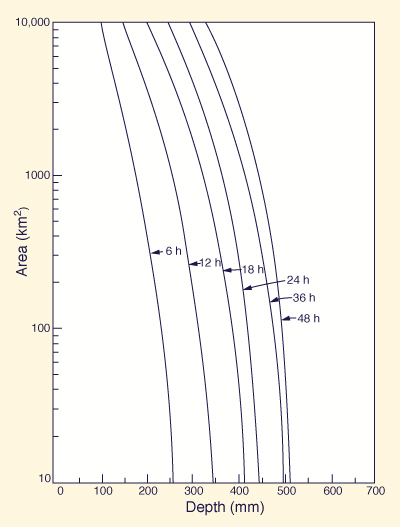
DAD analysis can also be used to study regional rainfall characteristics. Table 2-2 shows maximum DAD data for the United States, based on four extreme events. The data confirm that storm depth increases with duration and decreases with catchment area.
| |||||||||||||||||||||||||||||||||||||||||||||||||||||||||||||||||||||||||||||||||||||||
Probable Maximum Precipitation. For large projects, storm analysis using depth-duration-frequency data is not sufficient to eliminate the likelihood of failure. In such cases, the concept of PMP is used instead. In the United States, PMP estimates are developed following guidelines included in the HM NOAA Hydrometeorological Reports) serie [33-44] and related publications [84-87]. These reports contain methodologies and maps for the estimation of PMP or a given geographic location, range of durations and catchment sizes, and time of the year (Chapter 14).
Geographic and Seasonal Variations of Precipitation
Precipitation varies not only temporally and spatially but also seasonally, annually, and with geographic location and climate. Mean annual precipitation, the total amount of precipitation that accumulates in one year, on the average, at a given location, is used for classify climates (in terms of precipitation) into eight classes [11*]:
- Superarid: Less than 100 mm
- Hyperarid: 100 - 200 mm
- Arid: 200 - 400 mm
- Semiarid: 400 - 800 mm
- Subhumid: 800 - 1600 mm
- Humid: 1600 - 3200 mm
- Hyperhumid: 3200 - 6400 mm.
- Superhumid: More than 6400 mm.
The seasonality of precipitation is assessed with the precipitation seasonality index: the ratio of accumulated precipitation for the three wettest consecutive months to that for the three driest consecutive months, in an average year. This index is used to classify climates into four classes [11]:
- Nonseasonal: 1.0 - 1.6
- Weakly seasonal: 1.6 - 2.5
- Moderately seasonal: 2.5 - 10
- Strongly seasonal: Greater than 10.
In general, arid and semiarid climates are associated with moderately seasonal regimes; conversely, subhumid and humid climates are associated with weakly seasonal or nonseasonal regimes. However, there are some exceptions; for instance, the monsoon-type climates which prevail in some parts of the world, which tend to be both humid and seasonal.
Precipitation Data Sources and Interpretation
Precipitation data are obtained by measurement using rain gages (Chapter 3). The National Climatic Data Center (NCDC), Asheville, North Carolina, publishes precipitation data for about 8000 stations in the United States. A large number of additional gages are operated by other federal, state, and local agencies, and by individuals. U.S. federal agencies collecting precipitation data on a regular basis include the National Weather Service (NWS), the Army Corps of Engineers, the Natural Resources Conservation Service (formerly Soil Conservation Service), the Forest Service, the Bureau of Reclamation, and the Tennessee Valley Authority.
NCDC assembles precipitation data using hourly, daily, monthly, and yearly intervals. Hourly precipitation data and maximum 15-minute duration amounts are found in Hourly Precipitation Data. Daily and monthly precipitation data are found in Climatological Data. Monthly and annual precipitation data for about 250 major U.S. cities, including hourly rates, are found in Local Climatological Data.
Regional precipitation-frequency atlases (U.S. Weather Bureau No. 40 [86], NOAA Technical Memorandum NWS Hydro-35 [59] and Precipitation Frequency Atlas of the Western United States [58] are avaIlable. NCDC Monthly and seasonal precipitation maps are found in Weekly Weather and Crop Bulletin, available from NOAA/USDA Joint Agricultural Weather Facility, in the USDA South Building, Washington, D.C. Additional sources of precipitation data are given in Annotated Bibliography of NOAA Publications of Hydrometeorological Interest, updated at regular intervals by NWS, and in Selective Guide to Climatic Data Sources, updated at regular intervals by NCDC.
Precipitation and other relevant climatological data are now accessible online through NCDC's website at http://www.ncdc.noaa.gov. Clicking on On-line Data Access provides access to a host of on-line services, including U.S. monthly precipitation for NWS and Cooperative sites, and the On-line Access and Service Information System (OASIS), which includes hourly and 15-minute precipitation data.
Filling In Missing Records. Incomplete records of rainfall are sometimes possible due to operator error or equipment malfunction. In this case, it is often necessary to estimate the missing record. Assume that a certain station X has a missing record. A procedure to fill in the missing record is to identify three index stations (A, B, and C) having complete records, located as close to and as evenly spaced around station X as possible. The mean annual rainfall for each of the stations X, A, B, and C is evaluated. If the mean annual rainfall at each of the index stations A, B, or C is within 10 percent of that of station X, a simple arithmetic average of the rainfall values at the index stations provides the missing value at station X.
If the mean annual rainfall at any of the index stations differs by more than 10% from that of station X, the normal ratio method is used [55]. In this method, the missing precipitation value at station X is the following:
|
NX NX NX PX = (1/3) [ _____ PA + _____ PB + _____ PC ] NA NB NC | (2-10) |
in which P = precipitation, N = mean annual rainfall, and the subscripts X, A, B, and C refer to the respective stations.
An alternate method for filling in missing precipitation data has been developed by the National Weather Service [49]. The method requires data for four index stations A, B, C, and D, each located closest to the station X of interest, and in each of four quadrants delimited by north-south and east-west lines drawn through station X (Fig. 2-15). The estimated precipitation value at station X is the weighted average of the values at the four index stations. For each index station, the applicable weight is the reciprocal of the square of its distance L to station X.
Fig. 2-15 Position of station X and index stations A, B, C, and D. |
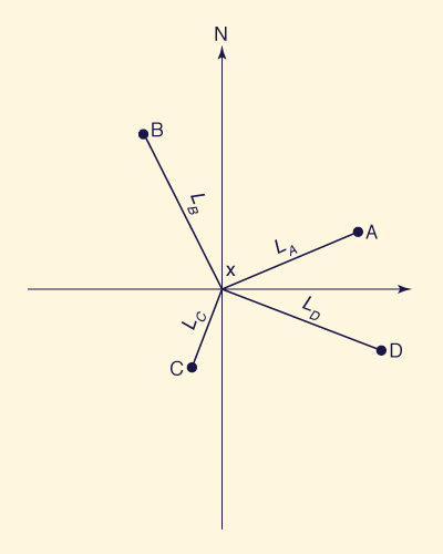
The procedure is described by the following formula:
|
4 Σ ( Pi / Li 2 ) i = 1 PX = _____________________ 4 Σ ( 1 / Li 2 ) i = 1 | (2-11) |
in which P = precipitation; L = distance between index stations and station X; and I refers to each one of the index stations A, B, C, and D.
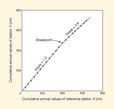
Double-mass Analysis. Changes in the location or exposure of a rain gage may have a significant effect on the amount of precipitation it measures, leading to inconsistent data (data of different nature within the same record).
The consistency of a rainfall record is tested with double-mass analysis. This method
compares the cumulative annual (or, alternatively, seasonal) values of station Y with
those of a reference station X. The reference station is usually the mean of several
neighboring stations. The cumulative pairs (double-mass values) are plotted in an x-y
arithmetic coordinate system, and the plot is examined for trend changes. If the plot is
essentially linear, the record at station Y is consistent. If the plot shows a break in slope,
the record at station Y is inconsistent and should be corrected. The correction is
performed by adjusting the records prior to the break to reflect the new state (after the
break). To accomplish this, the rainfall records prior to the break are multiplied by the
ratio of slopes after and before the break (Fig. 2-16).
Fig. 2-16 Double-mass analysis. |
2.2 HYDROLOGIC ABSTRACTIONS
|
|
Hydrologic abstractions are the processes acting to reduce total precipitation into effective precipitation. Effective precipitation eventually produces surface runoff. The difference between total and effective precipitation is the depth abstracted by the catchment.
The processes by which precipitation is abstracted by the catchment are many. Those important in engineering hydrology are the following:
- Interception,
- Infiltration,
- Surface or depression storage,
- Evaporation, and
- Evapotranspiration.
Interception
Interception is the process by which precipitation is abstracted by vegetation or other forms of surface cover, including, in certain cases, cultural features of the landscape. Interception loss is the fraction of precipitation that is retained by the vegetative cover. The intercepted amount is either returned to the atmosphere through evaporation, or go on to constitute throughfall, that part of precipitation which reaches the ground by first passing through the vegetative cover. Interception losses are a function of:
- Storm character, including intensity, depth, and duration,
- The type, species, age, and density of vegetative cover, and
- The time of the year, or season.
Interception is usually the first abstractive process to act during a storm. Light storms are substantially abstracted by the interception process. Light storms occur frequently and therefore constitute the majority of the storms. The interception loss accumulated in one year, primarily from light storms, amounts to about 25 percent of the average annual precipitation.
For moderate storms, interception losses are apt to vary widely, being greater during the growing season and smaller at other times of the year. Studies have shown that interception values are likely to vary from 7 to 36 percent of total precipitation during the growing season, and from 3 to 22 percent during the remainder of the year [12].
For heavy storms, interception losses usually amount to a small fraction of the total rainfall. For long-duration or infrequent storms, the effect of interception on the overall process of abstraction is likely to be small. In certain cases, particularly for flood hydrology studies, the neglect of interception is generally justified on practical grounds.
The interception loss comprises two distinct elements [25] The first is the interception storage, i.e., the depth (or volume) retained in the foliage against the forces of wind and gravity. The second is the evaporation loss from the foliage surface, which takes place throughout the duration of the storm. The combination of these two processes leads to the following formula for estimating interception loss [12].
|
L = S + K E t | (2-12) |
in which L = interception loss, in millimeters; S = interception storage depth in millimeters, usually varying from 0.25 to 1.25 mm; K = ratio of evaporating foliage surface to its horizontal projection; E = evaporation rate in millimeters per hour; and t = storm duration, in hours.
Infiltration
Infiltration is the process by which precipitation is abstracted by seeping into the soil below the land surface. Once below the ground surface, the abstracted water moves either laterally, as interflow, into lakes, streams, and rivers, or vertically, by percolation, into aquifers. The water that reaches lakes either evaporates or drains as lake overflow into surface streams. The water that reaches streams and rivers moves relatively rapidly toward the oceans as surface flow. The water held in aquifers moves slowly as groundwater flow, eventually flowing into a stream or reaching the ocean directly, bypassing the surface waters entirely.
Infiltration is a complex process. It is described by either an instantaneous or an average infiltration rate, both measured in millimeters per hour, or inches per hour. The total infiltration depth is obtained by integrating the instantaneous infiltration rate over the storm duration. The average infiltration rate is obtained by dividing the total infiltration depth by the storm duration.
Infiltration rates vary widely, depending on:
- The condition of the land surface, including compaction and surface crusting,
- The type and density of vegetative cover, and associated root structure,
- The physical properties of the soil, including structure, grain size, and gradation,
- The storm character, i.e., intensity, depth, and duration,
- The water temperature, and
- The water quality, including chemical constituents and other impurities.
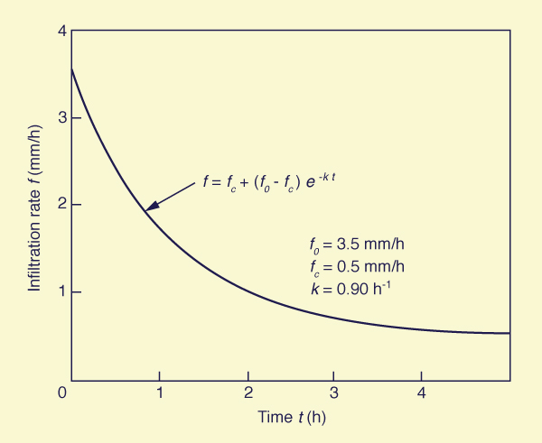
Infiltration Formulas. For a given storm, infiltration rates tend to vary in time. The initial infiltration rate is the rate prevailing at the beginning of the storm. This rate is likely to be the maximum rate for the given storm, gradually decreasing as the storm progresses in time. For storms of long duration, the infiltration rate eventually reaches a constant value, referred to as final (or equilibrium) infiltration rate. This process led Horton [27] to describe the variation of infiltration rate with time using the following formula:
| f = fc + ( fo - fc ) e-k t | (2-13) |
in which f = instantaneous infiltration rate; fo = initial infiltration rate;
fc = final infiltration rate; k = an exponential decay
constant; and t = time, in hours.
The units of k are h-1.
For t = 0, f = fo; and for t = ∞, f
= fc (see Fig. 2-17).
Fig. 2-17 Horton's infiltration formula. |
Equation 2-13 has three parameters: (1) initial infiltration rate; (2) final infiltration rate; and (3) the k value describing the rate of decay of the difference between initial and final infiltration rates. Field measurements are necessary in order to determine appropriate values of these parameters. A plot of infiltration rate versus time enables the estimation of the final rate. With a knowledge of the final rate, two sets of I and t are obtained from the plot and used, together with Eq. 2-13, to solve simultaneously for fc and k.
Integrating Eq. 2-13 between t = 0 and t = ∞, leads to:
|
fo - fc F = _________ k | (2-14) |
in which F = the total infiltration depth above the f = fc line. Equation 2-14 enables the calculation of the total infiltration depth, assuming that the storm lasts long enough for the equilibrium rate to be attained.
Example 2-2.
Assuming fo = 10 mm/h, fe = 5 mm/h, and k = 0.95 h-1,
calculate the total infiltration depth for a storm lasting 6 h.
After 6 h, the difference between instantaneous and
final rates is negligible. Therefore, the total infiltration depth is: (10 mm/h - 5 mm/h)/ 0.95 h-1 + (5 mm/h × 6 h)
= 35.26 mm. |
Typical infiltration rates at the end of 1 h (f1) are shown in Table 2-4. Generally, these values are reasonable approximations of final (i.e., equilibrium) infiltration rates.
| |||||||||||||||
More recent developments in infiltration theory have sought to improve on the Horton model. Philip [66] has proposed the following model:
| f = (l/2 ) s t -1/2 + A | (2-15) |
in which f = instantaneous infiltration rate; s = an empirical parameter related to the rate of penetration of the wetting front (the wetting surface characterized by a very high potential gradient); A = an infiltration value that is close to the value of saturated hydraulic conductivity at the surface; and t = time.
In Eq. 2-15, for t = 0, f = ∞; and for t = ∞, f = A. In practice, the initial infiltration rate has a finite value. In spite of this limitation, the Philip formula seems to be a good fit to experimental data. Integration of the Philip equation leads to
| F = s t 1/2 + A t | (2-16) |
in which F = total depth of infiltration.
An infiltration model with a sound theoretical basis is the Green and Ampt formula [21]. This equation describes infiltration rate under ponded water conditions as follows:
|
H + Pf f = K ( 1 + __________ ) Zf | (2-17) |
in which f = infiltration rate in millimeters per hour; K = saturated hydraulic conductivity in millimeters per hour; H = depth of ponded water in millimeters; Pf = capillary pressure at the wetting front in millimeters; and Zf = vertical depth of saturated zone in millimeters. In practice, however, it may be difficult to measure some of the terms of this equation. Recent progress has been achieved by groupe terms in Eq. 2-17 into predictable parameters linked to the physical processes [48].
Infiltration Indexes. Practical evaluations of infiltration have been hampered by its spatial and temporal variability. This has led to the use of infiltration indexes, which model the infiltration process in an approximate yet practical way.
Infiltration indexes assume that infiltration rate is constant throughout the storm duration. This assumption tends to underestimate the higher initial rate of infiltration while overestimating the lower final rate. For this reason, infiltration indexes are best suited for applications involving either long-duration storms or catchments with high initial soil moisture content. Under such conditions, the neglect of the variation of infiltration rate with time is generally justified on practical grounds.
For moderate storms, the use of infiltration indexes is largely an empirical procedure, with attention being focused on matching the prevailing soil moisture condition and storm duration in order to effect a proper balance of rainfall and runoff amounts.
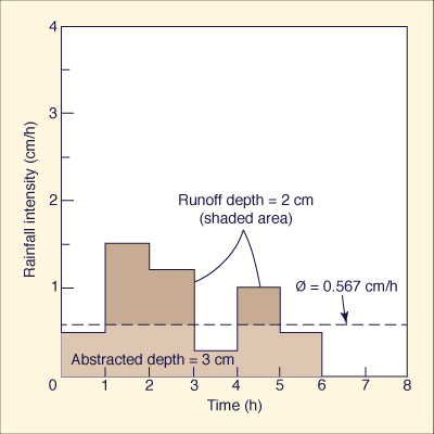
In practice, the most commonly used infiltration index is the φ-index, defined as the (constant) infiltration rate to be subtracted from the prevailing rainfall rate in order to obtain the runoff volume that actually occurred [13]. The computation of the φ-index requires a storm pattern, i.e., a plot of rainfall intensity versus time, and a measured runoff volume (or depth). The computation involves a trial-and-error procedure.
|
Example 2-3.
The runoff depth has been estimated at 2 cm. Calculate the φ-index.
From the rainfall distribution, the total rainfall is 5 cm. Therefore, the depth
abstracted by infiltration is:
[ (1.5 - φ) × 1 ] + [ (1.2 - φ) × 1 ] + [ (1.0 - φ) × 1 ] = 2 cm
From Eq. 2-18, solving for φ gives: φ = 0.567 cm/h, verifying that the assumed range
for was correct. Had the assumed range been wrong, the calculated φ-value would have been
out of that range. In Fig. 2-18, the 2 cm of runoff are above the φ-index line; the 3 cm
of abstracted rainfall are below the φ-index line. |
Fig. 2-18 Calculation of φ-index: Example 2-3. |
Another widely used infiltration index is the W-index [13], which, unlike the φ-index, takes explicit account of interception loss and depth of surface storage. The formula for the W-index is the following:
|
P - Q - S W = _____________ tf | (2-18) |
in which W = W-index, in millimeters per hour; P = rainfall depth, in millimeters; Q = runoff depth, in millimeters; S = the sum of interception loss and depth of surface storage, in millimeters; and tf = the total time (hours) during which rainfall intensity is greater than W.
The Wmin index is the W-index calculated for extremely wet conditions. It is derived using data from the last of a series of storms and is used in estimating maximum flood potential. In this sense, the Wmin index approaches a spatially averaged value of the final infiltration rate. For such extreme conditions, the values of Wmin and φ are almost identical.
Infiltration Rates Derived from Rainfall-Runoff Data. Inflltration formulas depict the variation of infiltration rates with time. Infiltration rates, however, vary not only temporally but also spatially. Unless the field measurements and related parameter estimation are fairly good representations of the spatial variability, the rates calculated by infiltration formulas are likely to be different from reality.
This difficulty is circumvented by calculating infiltration rates indirectly, from concurrent rainfall-runoff measurements. Such a calculation provides a temporal and spatial average of infiltration rate, amounting to a φ-index, with its associated advantages and disadvantages.
Infiltration and Catchment Size. For midsize and large catchments, the natural variability of infiltration rates makes it necessary to resort to the evaluation of total infiltration depth. In practice, total infiltration depths are derived from rainfall-runoff analysis. However, for each data set, the calculation is highly dependent on the level of soil moisture antecedent to the storm. The catchment moisture level is referred to as the antecedent moisture condition, or AMC (Chapter 5). Initial infiltration rates and, consequently, total infiltration depths are a function of prevailing antecedent moisture condition.
Surface or Depression Storage
Surface (or depression) storage is the process by which precipitation is abstracted by being retained in puddles, ditches, and other natural or artificial depressions of the land surface. Water held in depressions either evaporates or eventually contributes to soil moisture by infiltration. The spatial variability of storage in surface depressions precludes its precise calculation.
Intuitively, the milder the catchment's relief, the greater the effect of depression storage. Field data reported by Viessman [82] showed conclusively that depression storage is inversely related to catchment slope. Usually, an equivalent depth of depression storage can be estimated based on experience. For instance, Hicks [23] has used depression storage depths of 5.0, 3.75, and 2.5 mm for sand, loam, and clay, respectively. Tholin and Keife [77] have used values of 6.25 mm in pervious urban areas and 1.5 mm for paved areas. Where accurate estimations are difficult, depression storage amounts can be lumped together with other more tractable hydrologic abstractions such as interception or infiltration.
An alternate way of accounting for depression storage is the use of a peak-flow correction factor, as in the NRCS TR-55 graphical method (Section 5.3).
Typically, the effect of depression storage varies in time and, consequently, with storm duration. At the beginning of a storm, depression storage usually plays an active role in abstracting precipitation amounts. As time progresses, depression storage volumes are eventually filled, with any additional water going on to constitute runoff. This has led to the following conceptual model of depression storage:
| Vs = Sd ( 1 - e - k Pe ) | (2-19) |
in which Vs = equivalent depth of depression storage, in millimeters; Pe = precipitation excess, defined as total precipitation depth minus interception loss minus total infiltration depth; Sd = depression storage capacity, in millimeters; and k = a constant.
Linsley et al. [53] have suggested that values of Sd for most catchments are in the range of 10-50 mm. The value of the constant k is estimated by assuming that for very small values of precipitation excess (Pe ≅ 0), essentially all the precipitation goes into depression storage (dVs /dPe = 1). This leads to k = 1/Sd.
Evaporation
Evaporation is the process by which water accumulated on the land surface (including that held in surface depressions and water bodies such as lakes and reservoirs) is converted into vapor state and returned to the atmosphere. Evaporation occurs at the evaporating surface, the contact between water body and overlying air. At the evaporating surface, there is a continuous exchange of liquid water molecules into water vapor and vice versa. In engineering hydrology, evaporation refers to the net rate of water transfer (loss) into vapor state.
Evaporation is expressed as an evaporation rate in millimeters per day (mm/d), centimeters per day (cm/d), or inches per day (in./d). Evaporation rate is a function of several meteorological and environmental factors. Those important from an engineering hydrology standpoint are:
- Net solar radiation,
- Saturation vapor pressure,
- Vapor pressure of the air,
- Air and water surface temperatures,
- Wind velocity, and
- Atmospheric pressure.
Evaporation rates are significantly affected by climate. Studies have shown that evaporation rates
are high in arid and semiarid regions and low in humid regions. For instance, mean annual lake evaporation in
the United States varies from 20 in. (508 mm) in the Northeast (Maine) and Northwest (Washington state) corners,
to more than
80 in.
(2184 mm) in the Southwestern desert (California and Arizona) (Fig. 2-19) [18].
Fig. 2-19 Mean annual lake evaporation in the contiguous United States (NOAA). |

The effect of climate on evaporation has a substantial impact on water resources development. The planning and design of storage reservoirs in arid/semiarid regions requires a detailed evaluation of the potential for reservoir evaporation. These calculations determine to a large extent the feasibility of building surface water storage projects on regions subject to high evaporation rates.
Unlike other phases of the hydrologic cycle, lake evaporation cannot be measured directly. Therefore, several approaches have been developed to calculate evaporation. These vary in nature and are based on either: (1) a water budget, (2) an energy budget, or (3) a mass-transfer methodology.
Water Budget Method for Determining Reservoir Evaporation. The water budget method assumes that all relevant water-transport phases can be evaluated for a time period Δt, and expressed in terms of volumes. Reservoir or lake evaporation is calculated as follows:
|
E = P + Q - O - I - ΔS | (2-20) |
in which E = volume evaporated from the reservoir, P = precipitation faIling directly onto the reservoir, Q = surface runoff inflow into the reservoir, O = outflow from the reservoir, I = net volume infiltrated from the reservoir into the ground, and ΔS = change in stored volume. All terms in Eq. 2-20 refer to a time period Δt, usually taken as 1 week or greater.
Most terms in Eq. 2-20 can be evaluated directly. Precipitation is readily measured, and inflow and outflow can be obtained by integrating the flow records. The change in stored volume is determined by means of water stage recorders. Net infiltration, however, can be evaluated only indirectly, either by measuring soil permeability or monitoring changes in groundwater level in nearby wells. The difficulty in measuring net infiltration generally limits the water budget method to areas with little or no net infiltration. In spite of this limitation, the water budget method has been found to work reliably under certain idealized conditions. Water budget studies from Lake Hefner, Oklahoma, show that the method can provide evaporation volumes within a 10 percent accuracy about two-thirds of the time [81]. Conditions at Lake Hefner, however, were highly selective, and lesser accuracy is to be expected under more typical circumstances.
Energy Budget Method for Determining Reservoir Evaporation. During evaporation, significant energy exchanges occur at the evaporating surface. A balance of these energy exchanges leads to the energy budget method of calculating reservoir evaporation. The amount of heat required to convert one gram of water into vapor, i.e., the heat of vaporization, varies with temperature. For instance, at 20°C the heat of vaporization is 586 calories (Table A-I, Appendix A). To maintain the temperature of the evaporating surface, large quantities of heat must be supplied by radiation, by heat transfer from the atmosphere, and from energy stored in the water body.
Radiation is the emission
of energy in the form of electromagnetic waves from all bodies above 0°K. Solar radiation
received on the Earth's surface is a major component of the energy balance. Solar
radiation reaches the outer surface of the atmosphere at a nearly constant flux of
about 1.95 cal/cm2/min, or langleys/min (1 langley = 1 cal/cm2), measured
perpendicular to the incident radiation. Nearly all this radiation is of wavelengths
in the range
Fig. 2-20 Range of visible light within the electromagnetic spectrum. |
In passage through the atmosphere, solar radiation changes its flux and spectral composition. Some of it is reflected back to space, and some of it is absorbed and scattered by the atmosphere. The fraction of the original solar radiation flux that reaches the Earth's surface is called direct solar radiation. The fraction of the radiation reflected and scattered by the atmosphere that reaches the ground is called sky radiation. The sum of direct solar radiation and sky radiation is called global radiation.
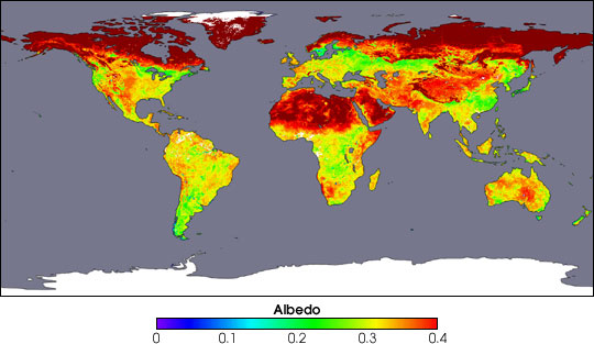
Albedo is the
reflectivity coefficient of a surface toward shortwave radiation. This coefficient varies
with color, roughness, and inclination of the surface. Its value is
| |||||||||||||||||||||||
Fig. 2-21 Global distribution of albedo (NASA). |
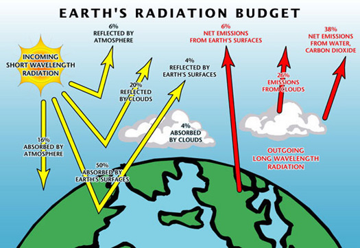
In addition to the shortwave radiation balance, there is also a longwave radiation
balance. The Earth's surface emits radiation, part of which is absorbed and reflected back
by the atmosphere. The difference between outgoing and incoming fluxes is called longwave
radiation loss. During the day, longwave radiation may be a small fraction of the total radiation
balance, but at night, in the absence of solar radiation, longwave radiation dominates the
radiation balance. Net radiation is equal to the net shortwave (solar) radiation minus the longwave (terrestrial) radiation toss (Fig. 2-22).
Fig. 2-22 The Earth's radiation budget (NASA). |
In the energy budget method, the incoming energy can be expressed as
|
Qi = Qs ( 1 - A ) - Qb + Qa | (2-21) |
in which Qi = incoming energy; Qs = global radiation (shortwave radiation from sun and sky); A = albedo; Qb = longwave radiation loss by water body; and Qa = net energy advected into the water body by streams, rain, and snow.
The energy expenditure, which must balance the incoming energy, is expressed as follows:
|
Qo = Qh + Qe + Qt | (2-22) |
in which Qo = energy expenditure; Qh = sensible heat transfer from water body to the atmosphere by convection and conduction; Qe = energy expended in the evaporation process; and Qt = increase in energy stored in the water body. The value of Qe is negative when condensation is taking place. All terms in Eqs. 2-21 and 2-22 are given in calories per square centimeter per day. The energy used in evaporation Qe (cal/cm2/day) is converted into equivalent evaporation rate E (cm/day) by the following formula:
|
Qe = ρ H E | (2-23) |
in which ρ = density of water in grams per cubic centimeter (g/cm3); H = heat of vaporization, a function of temperature (see Table A-1, Appendix A), in calories per gram (cal/g); and E = evaporation rate, in centimeters per day.
The terms Qh and Qe in Eq. 2-22 are difficult to evaluate directly. Bowen has suggested that their ratio is more tractable and can be evaluated by means of the following relation:
|
Qh Ts - Ta p B = _______ = γ ___________ _________ Qe es - ea 1000 | (2-24) |
in which B = Bowen's ratio, γ = a psychrometric parameter, which is a function of the physical properties of dry air, varying slightly with temperature (see Table 2-6); Ts = water surface temperature, in degrees Celsius; Ta = overlying air temperature, in degrees Celsius; es = saturation vapor pressure at the water surface temperature, in millibars; ea = vapor pressure of the overlying air, in millibars; and p = atmospheric pressure, in millibars.
A balance of incoming energy (Eq. 2-21) and energy expenditure (Eq. 2-22), taking into account Eqs. 2-23 and 2-24 leads to:
|
Qs ( 1 - A ) - Qb + Qa - Qt E = __________________________________ ρ H ( 1 + B ) | (2-25) |
The quantities Qs ( 1 - A ) and Qb can be measured with radiometers, which are instruments designed to measure radiation. The quantity Qa can be determined by measuring volumes and temperatures of the water flowing into and out of the body, and Qt is evaluated by periodic measurements of water temperatures. An example of the application of the energy budget method to a large lake is the study of evaporation in Lake Ontario by Bruce and Rodgers [9].
Mass-Transfer Approach. Evaporation rates are dependent on the water surlace temperature and the prevailing atmospheric pressure. Higher water surface temperatures induce more vigorous molecular action and result in higher evaporation rates. On the other hand, a higher atmospheric pressure limits the movement of water molecules and results in lower evaporation rates. In practice, the overall effect of atmospheric pressure on evaporation is small and is usually neglected.
The pressure at the air-water interface resulting from molecular motion in the direction of escape from the liquid is called the water vapor pressure. This pressure, which varies with the water temperature as shown in Tables A-1 and A- 2 (Appendix A), determines the rate at which water molecules escape to the air and become water-vapor molecules. Once in the air, the water-vapor molecules displace air molecules and contribute their share to the total atmospheric pressure. This share is called the partial vapor pressure.
When the partial vapor pressure in a given air volume (overlying a given water volume) is in equilibrium with the water vapor pressure, there is no net exchange of water molecules; consequently, the air volume is said to be saturated. A saturated air volume contains all the water vapor that it can hold. The vapor pressure of a saturated air volume is called the saturation vapor pressure. This pressure varies with the air temperature and is identical to the water vapor pressure at that temperature.
The higher the temperature, the more water vapor a volume of air can hold, and the higher the saturation vapor pressure. The partial vapor pressure (of the air) ea is calculated by multiplying the saturation vapor pressure at the air temperature eo by the relative humidity, in percentage, and dividing by 100. Studies have shown that evaporation rates are a function of the difference between the saturation vapor pressure (expressed at the water surface temperature or, as an alternative, at the overlying air temperature) and the partial vapor pressure of the overlying air.
As the evaporation process continues, the lowest layer of the atmosphere eventually reaches saturation and the net evaporation rate decreases to zero and may actually reverse (condensation) (Fig. 2-23). Thus, an agent such as the wind, which opens up the system and carries away the water molecules as they leave the water surface, is necessary for evaporation to continue.
Fig. 2-23 Saturation vapor pressure analog. |

The recognition of these processes led Dalton [15] to formulate the classical law bearing his name:
|
E = f (u) ( es - ea ) | (2-26) |
in which E = evaporation rate; f(u) = a function of the horizontal wind speed; es = the saturation vapor pressure at the water surface temperature; and ea = the (partial) vapor pressure of the overlying air. When the air is saturated, i.e., when the relative humidity φ approaches 100%, ea is nearly equal to es, and the evaporation E tends to zero.
Several empirical equations of the type of Eq. 2-26 have been developed over the years. Collectively, they are referred to mass-transfer equations. A commonly used mass-transfer equation is that of Meyer [54]:
|
E = C ( eo - ea ) [ 1 + ( W / 10 ) ] | (2-27a) |
in which E = evaporation rate in inches per month; C = a coefficient varying from 15 for small ponds to 11 for large lakes and reservoirs; eo = saturation vapor pressure at the mean monthly air temperature, in inches of mercury; ea = vapor pressure of the air at the mean monthly air temperature, in inches of mercury; and W = mean monthly wind speed at 25-ft height, in miles per hour.
Another version of the Meyer equation is the following [55, 82]:
|
E = C ( es - ea ) [ 1 + ( W / 10 ) ] | (2-27b) |
in which E = evaporation rate, in inches per day; C = a coefficient varying from 0.50 for small ponds to 0.36 for large lakes and reservoirs; es = saturation vapor pressure at the daily water surface temperature, in inches of mercury; ea = vapor pressure of the air at the daily air surface temperature, in inches of mercury; and W = daily mean wind speed at 25-ft height, in miles per hour.
A set of mass-transfer equations developed in connection with the Lake Hefner evaporation studies [81] is the following:
|
E = 0.00304 ( es - e2 ) v4 | (2-28a) |
| E = 0.00241 ( es - e8 ) v8 | (2-28b) |
in which E = evaporation rate in inches per day; es = saturation vapor pressure at the (daily) water surface temperature in inches of mercury; e2 and e8 are partial (air) vapor pressures over the lake at 2- and 8-m heights, respectively, in inches of mercury; and v4 and v8 are wind speeds over the lake at 4- and 8-m heights, respectively, in miles per day. If e2 and v4 are taken upwind from the lake, the constant in Eq. 2-29a reduces to 0.0027. These formulas were carefully developed using water budget data from Lake Hefner, with a surface area of 2500 ac (1012 ha). They have since been tested other reservoirs, including Lake Mead and others in the western United States [10].
Combination Methods for Determining Reservoir Evaporation. The concurrent use of both of energy budget and mass-transfer approaches leads to an alternate way of determining reservoir evaporation. Penman [64] combined these two concepts to develop a formula for practical use. An approximate energy balance (neglecting variations of energy by the water body, Qa = 0, and Qt = 0, in Eqs. 2-21 and 2-22) led Penman to the following relation:
|
Qs ( 1 - A ) - Qb = Qh + Qe | (2-29) |
The left side of this equation is the net radiation, or Qn. The right side can be expressed in terms of the Bowen ratio (Eq. 2-24) as Qe ( 1 + B ). Therefore:
|
Qn = Qe ( 1 + B ) | (2-30) |
By using Eq. 2-23, Eq. 2-30 is converted to evaporation rate units (centimeters per day):
|
En = E ( 1 + B ) | (2-31) |
in which En is the evaporation rate due to net radiation, and E is the evaporation rate.
For p = 1000 mb, which is close to atmospheric pressure at sea level, equal to 1013.2 mb, Bowen's ratio (Eq. 2-24) reduces to:
|
Ts - Ta B = γ __________ es - ea | (2-32) |
A saturation vapor-pressure gradient Δ between surface water and overlying air temperatures, in millibars per degree Celsius, is defined as follows:
|
es - eo Δ = ___________ Ts - Ta | (2-33) |
in which es = saturation vapor pressure at the water surface temperature Ts, and eo = saturation vapor pressure at the overlying air temperature Ta.
The Dalton formula (Eq. 2-26) enables the calculation of the ratio
|
Ea eo - ea ______ = ___________ E es - ea | (2-34) |
Combining Eqs. 2-31 through 2-34, the Penman equation is obtained:
|
Δ En + γ Ea E = __________________ Δ + γ | (2-35) |
in which E (evaporation rate), En (evaporation rate due to net radiation) and Ea (mass-transfer evaporation rate) are given in centimeters per day; and Δ and γ are given in millibars per degree Celsius.
The quantities Δ and γ in Eq. 2-35 are weighting factors, affecting the net radiation and mass-transfer evaporation rates, respectively. The gradient Δ is a function of saturation vapor pressure and air temperature (Eq. 2-33). A simple formula based solely on air temperature is [53]:
|
Δ = ( 0.00815 Ta + 0.8912 )7 | (2-36) |
in which Δ is given in millibars per degree Celsius, and Ta = air temperature, in degrees Celsius. This formula is applicable for air temperatures greater than -25 oC.
The psychrometric parameter γ is directly proportional to atmospheric pressure and inversely proportional to the latent heat of vaporization. At standard (sea level) atmospheric pressure, γ varies slightly with temperature, as shown in Table 2-6.
Equation 2-35 can also be expressed as follows:
|
α En + Ea E = ________________ α + 1 | (2-37) |
in which α = Δ/γ, a function of air temperature. Values of α (with Δ based on Eq. 2-36) are shown in Table 2-6.
| ||||||||||||||||||||||||||||||||||||
The mass-transfer evaporation rate Ea is evaluated with an appropriate mass transfer equation. For instance, the following formula has been proposed by Dunne [17]:
|
100 - φ E = ( 0.013 + 0.00016 v2 ) eo ____________ 100 | (2-38) |
in which Ea = mass-transfer evaporation rate, in centimeters per day; v2 = wind velocity, measured at a 2-m depth, in kilometers per day; eo = saturation vapor pressure at the overlying air temperature, in millibars; and φ = relative humidity, in percent.
Other Penman-type equations have been developed over the past 50 years. For instance, the National Weather Service has developed a Penman-type equation for estimating evaporation based on mean daily air temperature and dew point, wind movement per day, and solar radiation [49, 51]. More recent examples are represented by the Penman-Monteith [56] and Shuttleworth-Wallace equations [74] (see following section: Evapotranspiration).
Example 2-4.
|
Evaporation Determinations Using Pans. Uncertainty in the applicability of the various evaporation formulas has led to the indirect measurement of evaporation using evaporation pans. An evaporation pan is a device designed to measure evaporation by monitoring the loss of water in the pan during a given time period, usually 1 d. It provides a measurement of the integrated effect of net radiation, wind, temperature and humidity on the evaporation from an open surface.
Evaporation pans vary widely in size, shape, materials, and exposure. The pan measurement is likely to be somewhat different from the actual amount of lake evaporation. The ratio of pan-to-Iake evaporation is an empirical constant referred to as the pan coefficient. Evaporation measurements using pans are discussed in Chapter 3.
Evapotranspiration
Evapotranspiration is the process by which water in the land surface, soil, and vegetation is converted
into vapor state and returned to the atmosphere. It consists of evaporation from water, soil, vegetative,
and other surfaces and includes transpiration by vegetation. In this sense, evapotranspiration encompasses
all the water converted into vapor and returned to the atmosphere and, therefore, it is an important component
in the long-term water balance of a catchment.
Fig. 2-24 Evapotranspiration. |

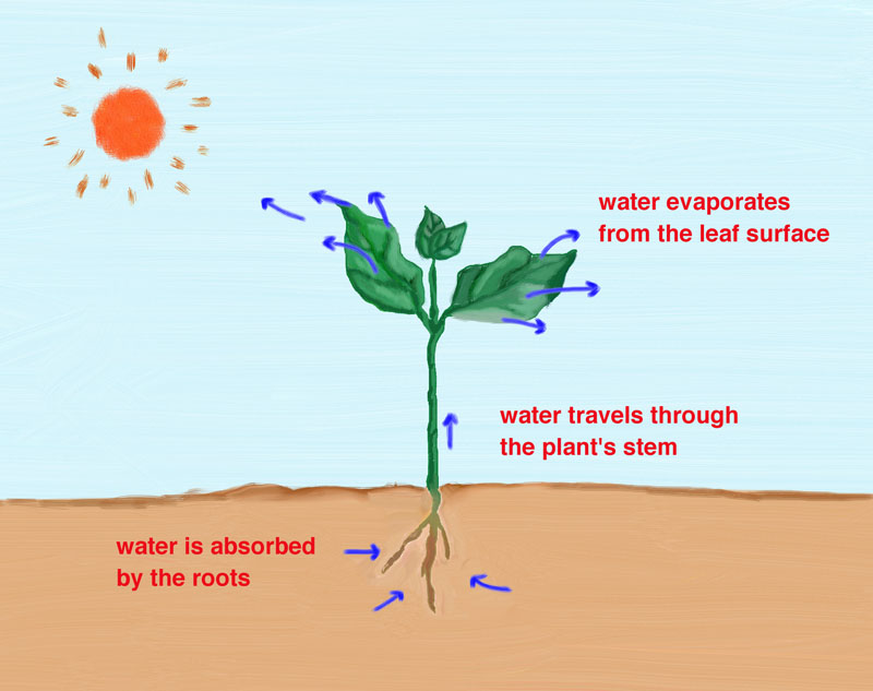
Transpiration is the process by which plants transfer water from the root zone to the leaf surface, where it eventually evaporates into the atmosphere. The process by which transpiration takes place can be described as follows:
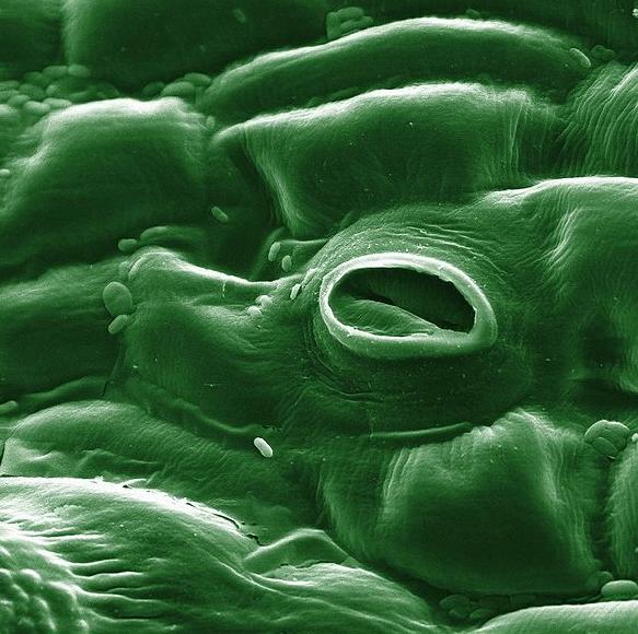
Osmotic pressures at the root zone act to move water into the roots. Once inside the root, water is transported through the plant stem to the intercellular spaces located within the leaves. Air enters the leaves through small surface openings called stoma, plural stomata (Fig. 2-25). Chloroplasts within the leaves use carbon dioxide from the air and a small portion of the available water to manufacture the carbohydrates necessary for plant growth. As air enters the leaf, water escapes through the open stomata and reaches the leaf surface, where it becomes available for evaporation.
The
ratio of water transpired and eventually vaporated to that actually used in plant growth is very large,
up to 800:1 or more [53].
Fig. 2-25 Stoma in a tomato leaf seen through |
Transpiration is a part of plant life and, therefore, it is a continuous process, occurring with or without the presence of precipitation. During a storm, however, interception amounts may use some of the energy available for evaporation, thereby reducing the amount of transpiration. The extent of this effect varies with vegetation type.
Transpiration is also limited by the rate at which moisture becomes available to the plants. Some authorities believe that transpiration is independent of the available soil moisture as long as the latter is above the permanent wilting point, i.e., the soil moisture at which permanent wilting would occur. Others assume that transpiration is roughly proportional to the prevailing soil moisture.
Transpiration rates and amounts vary
widely, depending on vegetation type, depth of root zone, and extent and density of vegetative cover (Fig. 2-26).
Measurements of transpiration are difficult and are usually possible only under highly controlled
circumstances. Since transpiration results in evaporation, transpiration amounts are a function of the
same meteorological and climatic factors that control evaporation rates. In practice, transpiration is
combined with evaporation and expressed as evapotranspiration, which includes all the water converted
into vapor and returned to the atmosphere.
Fig. 2-26 Transpiration. |
In evapotranspiration studies, the concept of potential evapotranspiration (PET) attributed to Thornthwaite [78] is widely used. Potential evapotranspiration is the amount of evapotranspiration that would take place under the assumption of an ample supply of moisture at all times. Therefore, PET is an indication of optimum crop water requirements.
Doorenbos and Pruitt [16] introduced the concept of reference crop evapotranspiration ETo, which is similar to that of potential evapotranspiration. Reference crop evapotranspiration is the rate of evapotranspiration from an extended surface of 8- to 15-cm tall green grass cover of uniform height, actively growing, completely shading the ground, and not short of water. Therefore, the reference crop evapotranspiration can be taken as the potential evapotranspiration of the reference crop (short green grass).
Potential evapotranspiration is equivalent to the evaporation that would occur on a free water surface of extended proportions but of negligible heat storage capacity [50]. Therefore, methods used to calculate potential evapotranspiration resemble the methods used to calculate evaporation. Like evaporation, there are many methods of calculating potential evapotranspiration, each having its own range of applicability. Data requirements vary widely, reflecting the assumptions used in their development.
Most potential evapotranspiration formulas are empirical, dependent upon the known correlation between potential evapotranspiration and one or more meteorological or climatic variables such as radiation, temperature, wind velocity, and vapor pressure difference. Other formulas relate evapotranspiration to direct measurements of water losses using evaporation pans. Models of evapotranspiration and potential evapotranspiration can be grouped into:
- Temperature models,
- Radiation models,
- Combination models, and
- Pan-evaporation models.
It is noted that, when applied to a given set of conditions, the various potential evapotranspiration formulas usually give different estimates. These, however, do not vary widely, with the ratio of maximum and minimum estimates fluctuating throughout the year and rarely exceeding 2:1. As with any such calculation, regional or local experience is required when choosing an appropriate method to calculate potential evapotranspiration.
Temperature Models to Estimate Evapotranspiration. The Blaney-Criddle formula [5, 6] is typical of the temperature models for the estimation of evapotranspiration. The formula has been widely used to estimate crop water requirements. Its original version, applicable on a monthly basis, has the following form:
|
F = P T | (2-39) |
in which F = evapotranspiration for a given month, in inches; P = a day-length variable, defined as the ratio of the total daytime hours for a given month to the total daytime hours in the year, a function of latitude; and T = mean monthly temperature, in degrees Fahrenheit.
In SI units, applicable on a daily basis, the Blaney-Criddle formula is the following:
|
f = p ( 0.46 t + 8.13 ) | (2-40) |
in which f = daily consumptive use factor, in millimeters; p = the ratio of mean daily daytime hours for a given month to the total daytime hours in the year, as a percent, a function of latitude (Table A-3, Appendix A); and t = mean daily temperature for a given month in degrees Celsius.
For a given crop, the consumptive
water requirement is the amount of water required to meet its evapotranspiration needs without
being limited by lack of water. The consumptive water requirement is equal to the product of
consumptive use factor f times an empirical consumptive use crop coefficient
Consumptive
water requirements vary widely between climates having similar air temperatures and day lengths.
Therefore, the effect of climate on crop water requirements is not fully described by the
consumptive use factor f. The effect of climate can be incorporated into the crop coefficient
Doorenbos and Pruitt [16] have proposed a correction to the Blaney-Criddle formula to account for the following local climatic conditions:
- The effect of actual insolation time (the ratio n/N of actual to maximum possible bright sunshine hours),
- Minimum relative humidity φmin in percent (or RH%), and
- Daytime wind speed Ud (measured at a 2-m depth), in m/s.
|
ETo = a + b f | (2-41) |
in which ETo = reference crop evapotranspiration, and a and b are
intercept and slope, respectively, as shown in Fig. 2-27, for three chosen levels of actual
insolation time (low, medium, and high), minimum relative humidity (low, medium, and high),
and daytime wind speed (light, moderate, and strong).
Fig. 2-27 Doorenbos and Pruitt's modification of the Blaney-Criddle formula. |
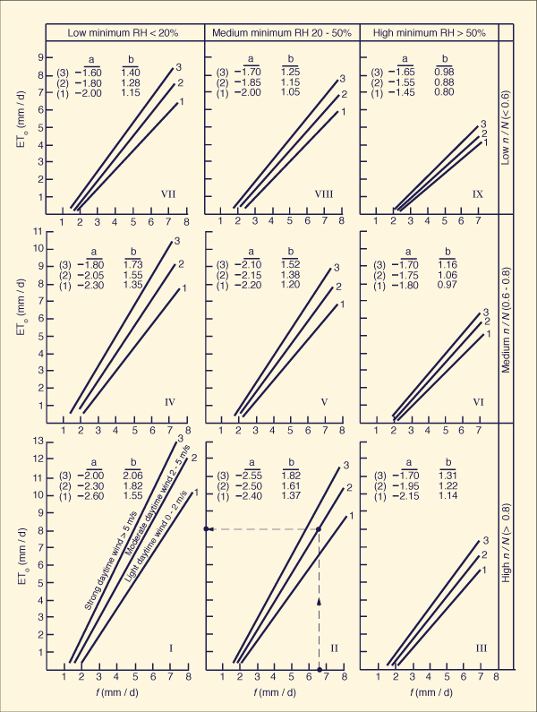
Based on Fig. 2-27, Frevert et al. [20] have developed regression equations for a and b:
|
The consumptive water requirement for a given crop, ETc , can be calculated as follows:
|
ETc = kc ETo | (2-42) |
Approximate range of seasonal crop coefficients are shown in Table 2-7.
|
| |||||||||||||||||||||||||||||||||||||||||||||||||||||||||||||||||||
Example 2-6.
|
The Thornthwaite method is another widely used temperature model to estimate potential evapotranspiration [78]. The method is based on an annual temperature efficiency index J, defined as the sum of twelve (12) monthly values of heat index I. Each index I is a function of the mean monthly temperature T, in degrees Celsius, as follows:
|
T I = ( _____ ) 1.514 5 | (2-43) |
Evapotranspiration is calculated by the following formula:
|
10 T PET (0) = 1.6 ( ______ ) c J | (2-44) |
in which PET (0) = potential evapotranspiration at 0o latitude, in centimeters per month; and c is an exponent to be evaluated as follows:
|
c = 0.000000675 J 3 - 0.0000771 J 2 + 0.01792 J + 0.49239
| (2-45) |
At latitudes other than 0o, potential evapotranspiration is corrected to:
|
PET = K PET (0) | (2-46) |
in which K is a constant for each month of the year, varying as a function of latitude (see Table A-4, Appendix A).
Example 2-7.
|
Radiation Models. Priestley and Taylor [67] proposed that potential evapotranspiration be taken as the radiation part of the Penman equation (Eq. 2-35 with Ea = 0) affected with an empirical constant. Priestley and Taylor's formula is the following:
|
1.26 Δ [ Qn / (ρ H ) ] PET = ________________________ Δ + γ | (2-47) |
in which PET = potential evapotranspiration, in centimeters per day; Qn = net radiation, in calories per square centimeter per day; Δ is the gradient defined by Eqs. 2-33 and 2-36; and γ is the psychrometric parameter (Table 2-6). Equation 2-47 can also be expressed as follows:
|
1.26 α [ Qn / (ρ H ) ] PET = ________________________ α + 1 | (2-47) |
in which the constant α can be obtained from Table 2-6.
Recent evaluation of the Priestley-Taylor formula has confirmed its applicability to humid climates. For better estimates in arid climates, the value of the empirical constant should be taken as 1.74 instead of 1.26 [75].
Example 2-8.
|
Pan-evaporation Models.
Evaporation pans provide a measurement of the integrated effect of radiation,
wind, temperature, and humidity on evaporation from an open surface. Plants and vegetation respond to the
same climatic conditions, but several factors produce significant differences in the loss of water. The albedo from
water surfaces is in the range
The basic pan-evaporation formula is the following:
|
PET = Kp Ep | (2-48) |
in which PET = potential evapotranspiration; Kp = pan coefficient; and Ep = pan evaporation.
The most common evaporation pans are the NWS Class A pan and the Colorado sunken pan. The NWS Class A pan
is circular, 122 cm in diameter and 25.4 cm deep, made of galvanized iron (22 gage) or Monel® metal (0.8 mm).
The pan is mounted on a wooden open-frame platform with its bottom 15 cm above ground level. The soil is built
up to within 5 cm of the bottom of the pan, and the pan must be leveled. It is filled with water 5 cm below the
rim, and water level is maintained within 7.5 cm below the rim (Fig. 2-28).
Fig. 2-28 Class A evaporation pan (benmeadows.com). |
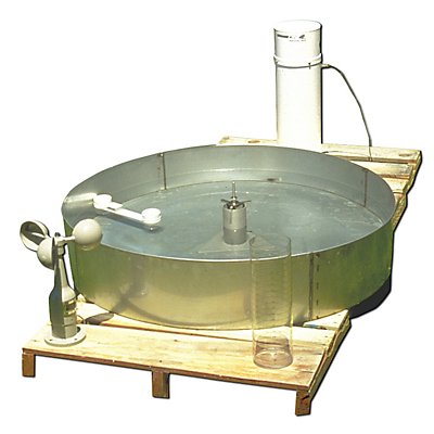
The Colorado sunken pan is sometimes preferred in crop water-requirement studies because these pans
tend to yield a better estimate of reference crop
evapotranspiration than the NWS Class A pan. The pan's cross section is a square of side 920 mm and depth 460 mm.
It is made of galvanized iron and set in the ground with the rim 50 mm above ground level (Fig. 2-29). The water inside the
pan is maintained at or slightly below ground level.
Fig. 2-29 Sketch of Colorado sunken pan. |
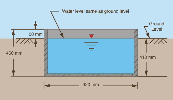
The pan evaporation approach has been widely used in the determination of potential evapotranspiration. Stanhill [76], for example, concluded that the Class A evaporation pan was the most promising method for estimating potential evapotranspiration. Doorenbos and Pruitt [16] have given guidelines for choosing an appropriate value of pan coefficient for several climatic and site conditions (see Table 2-8).
| |||||||||||||||||||||||||||||||||||||||||||||||||||||||||||||||||||||||||||||||||||||||||||||||||||||||||||||||||||||||||||||||||||||||||||||||||||||||||||||||||||||||||||||||||
2.3 CATCHMENT PROPERTIES
|
|
All
2.4 RUNOFF
|
|
The
QUESTIONS
|
|
Alley,
PROBLEMS
|
|
Alley,
REFERENCES
|
|
Alley, W. M., T. E. Reilly, and. O. E. Franke. 1999. Sustainability of ground-water resources. U.S. Geological Survey Circular 1186, Denver, Colorado, 79 p.
| http://engineeringhydrology.sdsu.edu | 140301 11:00 |