[Definition]   [Hydrologic Cycle]   [Catchment Budget]   [Uses]   [Approaches]   [Flood and Scale]   [Questions]   [Problems]   [References]   •   CHAPTER 1:   INTRODUCTION   "Unless the lower rivers are allowed to reassert their natural function as exporters of salt to the ocean, today's productive lands will eventually become salt encrusted and barren." Arthur F. Pillsbury (1981) This electronic book deals with principles of hydrologic science and their application to the solution of hydraulic, hydrologic, and water resources engineering problems, including the water-related environmental issues. This introductory chapter is divided into six sections. Section 1.1 defines hydrology and engineering hydrology. Section 1.2 describes the hydrologic cycle, a fundamental tenet of hydrologic science. Section 1.3 describes the closely related concepts of catchment and hydrologic budget. Section 1.4 explains the use of hydrologic knowledge in the solution of typical problems of hydraulic and hydrologic engineering. Section 1.5 elaborates on the various approaches used to solve problems of engineering hydrology. Section 1.6 discusses surface runoff, flood hydrology, and catchment scale. The concept of catchment scale is used in this book to develop a framework for the study of hydrologic models, methods, and techniques. 1.1  DEFINITION OF ENGINEERING HYDROLOGY [Hydrologic Cycle]   [Catchment Budget]   [Uses]   [Approaches]   [Flood and Scale]   [Questions]   [Problems]   [References]   •   [Top]   Hydrology is one of the earth sciences. It studies the waters of the earth, their occurrence, circulation and distribution, their chemical and physical properties, and their relation to living things. Hydrology encompasses surface water hydrology and groundwater hydrology; the latter, however, is considered to be a subject in itself. Other related earth sciences include climatology, meteorology, geology, geomorphology, sedimentology, geography, and oceanography. Engineering hydrology is an applied earth science. It uses hydrologic principles in the solution of engineering problems arising from human exploitation of the water resources of the Earth. In its broadest sense, engineering hydrology seeks to establish relations defining the spatial, temporal, seasonal, annual, regional, or geographical variability of water, with the aim of ascertaining societal risks involved in sizing hydraulic structures and systems. 1.2  THE HYDROLOGIC CYCLE [Catchment Budget]   [Uses]   [Approaches]   [Flood and Scale]   [Questions]   [Problems]   [References]   •   [Top]   [Definition]   The hydrologic cycle describes the continuous recirculatory transport of the waters of the earth, linking atmosphere, land, and oceans. The process is quite complex, containing many subcycles. To explain it briefly, water evaporates from the ocean surface, driven by energy from the sun, and joins the atmosphere, moving inland. Once inland, atmospheric conditions act to condense and precipitate water onto the land surface, where, driven by gravitational forces, it returns to the ocean through streams and rivers. Figure 1-1 shows a pictorial representation of the hydrologic cycle. A schematic view, including the interaction between the various phases and water-holding elements, is shown in Fig. 1-2 [2]. This schematic includes all physical processes relevant to engineering hydrology. Precipitation and other liquid-transport phases are represented by straight arrows, while evaporation and other vapor-transport phases are represented by wavy arrows. Fig. 1-1  The hydrologic cycle. 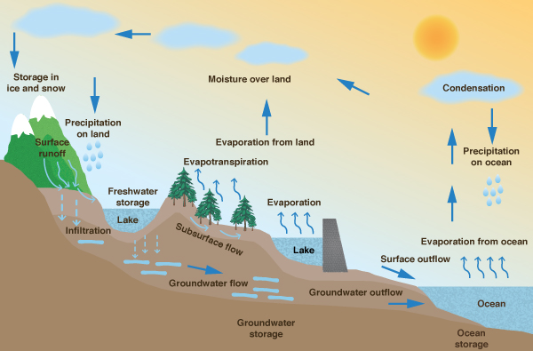Fig. 1.2  Schematic view of the hydrologic cycle (By permission from "Dynamic Hydrology," P. S. Eagleson, 1970, Mc-Graw-Hill [2]). 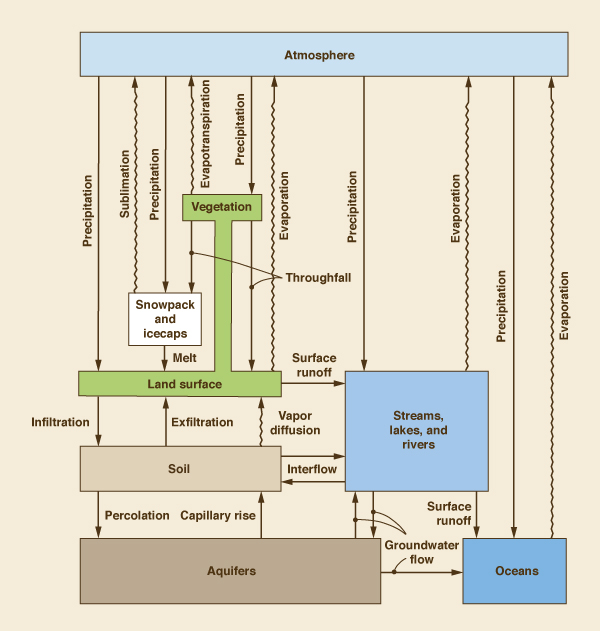The water-holding elements of the hydrologic cycle are: Atmosphere Vegetation Snowpack and icecaps Land surface Soil Streams, lakes, and rivers Aquifers Oceans. The liquid-transport phases of the hydrologic cycle are: Precipitation from the atmosphere onto land surface Throughfall from vegetation onto land surface Melt from snow and ice onto land surface Surface runoff from land surface to streams, lakes, and rivers, and from streams, lakes , and rivers to oceans Infiltration from land surface to soil Exfiltration from soil to land surface Interflow from soil to streams, lakes, and rivers and vice versa Percolation from soil to aquifers Capillary rise from aquifers to soil Groundwater flow from streams, lakes, and rivers to aquifers and vice versa, and from aquifers to oceans and vice versa. The vapor-transport phases of the hydrologic cycle are: Evaporation from land surface, streams, lakes, rivers, and oceans to the atmosphere Evapotranspiration from vegetation to the atmosphere Sublimation from snowpack and icecaps to the atmosphere Vapor diffusion from soil to land surface. 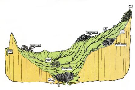1.3  THE CATCHMENT AND ITS BUDGET [Uses]   [Approaches]   [Flood and Scale]   [Questions]   [Problems]   [References]   •   [Top]   [Definition]   [Hydrologic Cycle]   A catchment is a portion of the earth's surface that collects runoff and concentrates it at its furthest downstream point, referred to as the catchment outlet (Fig. 1-3). The runoff concentrated by a catchment flows either into a larger catchment or into the ocean. The place where a stream enters a larger stream or body of water is referred to as the mouth. Fig. 1-3  The Upper Parramatta River catchment, New South Wales, Australia. In U.S. hydrologic practice, the terms watershed and basin are commonly used to refer to catchments. Generally, watershed is used to describe a small catchment (stream watershed), whereas basin is reserved for large catchments (river basins). In this book, the word catchment is used without a specific connotation of scale, whereas the use of the words watershed and basin follow established practice. 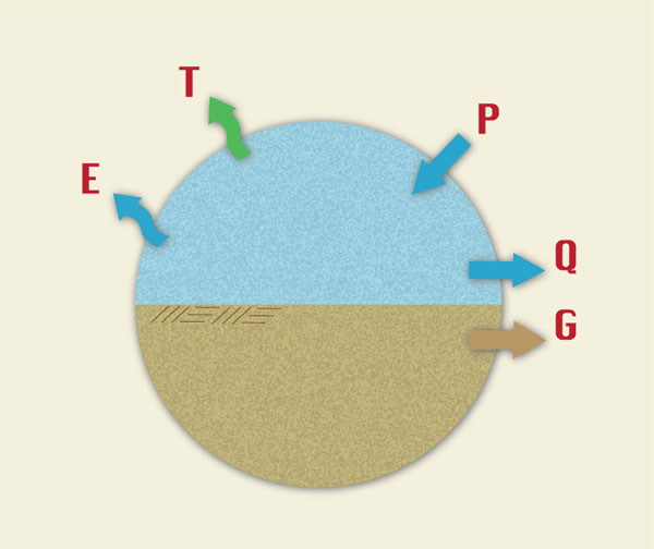The interpretation of the hydrologic cycle within the confines of a catchment leads to the concept of hydrologic budget. The hydrologic budget refers to an accounting of the various transport phases of the hydrologic cycle within a catchment, with the aim of ascertaining their relative magnitudes. The following is a hydrologic budget equation that considers both surface water and groundwater: ΔS = P - ( E + T + G + Q ) (1-1) in which ΔS = change in storage, P = precipitation, E = evaporation, T = evapotranspiration, G = groundwater outflow, and Q = surface runoff. Within a given time span, the change in water volume remaining in storage in a catchment is the difference between precipitation and the sum of evaporation, evapotranspiration, groundwater outflow, and surface runoff. In hydrologic practice, the terms of Eq. 1-1 are expressed in units of water depth, i.e., a water volume uniformly distributed over the catchment area. Under equilibrium conditions, ΔS = 0, and Eq. 1-1 reduces to (Fig. 1-4): P = E + T + G + Q (1-2) Fig. 1-4  A hydrologic budget that considers both surface water and groundwater. A hydrologic budget equation that considers only surface water is: ΔS = P - ( E + T + I + Q ) (1-3) in which I = infiltration, and all other terms have been already defined. Within a given time span, under equilibrium conditions, Eq. 1-3 reduces to (Fig. 1-5): P = E + T + I + Q (1-4) Fig. 1-5  A hydrologic budget that considers only surface water. 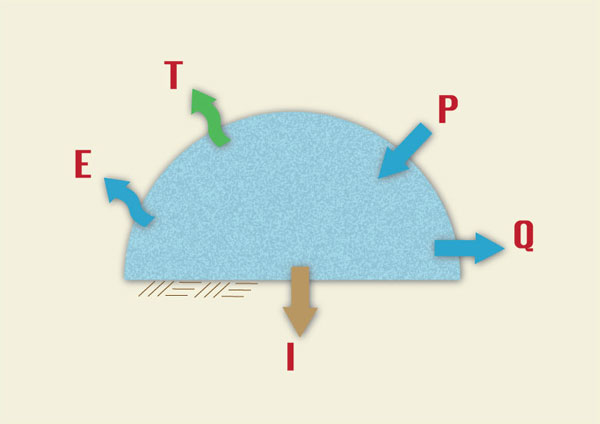Note that there may be some double counting in Eq. 1-4, because infiltration can convert into evaporation through lakes and wetlands, into evapotranspiration through vegetation, and into surface runoff (baseflow) through exfiltration. Equation 1-4 is often expressed in reduced form: Q = P - L (1-5) in which L = losses, or hydrologic abstractions, equal to the sum of evaporation E, evapotranspiration T, and infiltration I. Equation 1-4 states that runoff is equal to precipitation minus the aggregate of all losses. This concept is the basis of many practical methods of runoff computation (Chapters 4 and 5). 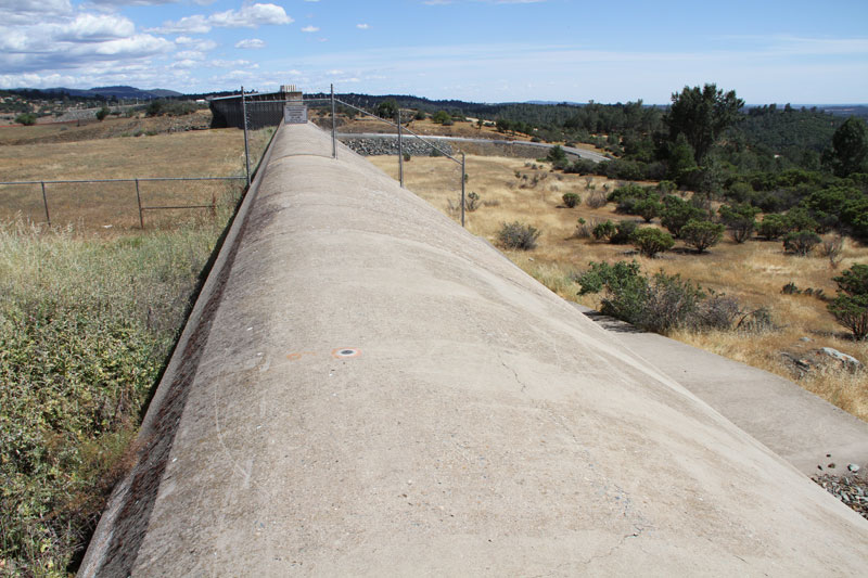1.4  USES OF ENGINEERING HYDROLOGY [Approaches]   [Flood and Scale]   [Questions]   [Problems]   [References]   •   [Top]   [Definition]   [Hydrologic Cycle]   [Catchment Budget]   Engineering hydrology seeks to answer questions of the following type: What is the maximum probable flood at a proposed or existing dam site (Fig. 1-6)? How does a catchment's water yield vary from season to season, and from year to year? What is the relationship between a catchment's surface water and groundwater resources? When evaluating low flow characteristics, what flow level can be expected to be exceeded 90 percent of the time? Given the natural variability of streamflows, what is the appropriate size of an instream storage reservoir? What hydrologic hardware (e.g., rainfall sensors) and software (computer models) are needed for real-time flood forecasting? In seeking answers to these questions, engineering hydrology uses analysis and measurement. Hydrologic analysis aims to develop a methodology to quantify a certain phase or phases of the hydrologic cycle, for instance, precipitation, infiltration, or surface runoff. The unit hydrograph technique (Chapter 5) is a good example of a time-tested method of hydrologic analysis. Field measurements such as stream gaging (Chapter 3) complement and verify the analysis. Statistical methods, e.g., linear regression (Chapter 7), supplement hydrologic analysis and/ or measurement. Generally, the hydrologic engineer is interested in describing either flow rates or volumes, including their spatial, temporal, seasonal, annual, regional, or geographical variability. Flow rates (discharges) are commonly expressed in cubic meters per second or cubic feet per second; volumes are expressed in cubic meters, cubic hectometers (1 hectometer is equal to 1 million cubic meters), or acre-feet. In engineering hydrology, volumes are often expressed in depth units (millimeters, centimeters, or inches), intended to represent a uniform water depth over the catchment area. Fig. 1-6  Emergency spillway at Oroville Dam, Northern California. 1.5  APPROACHES TO ENGINEERING HYDROLOGY [Flood and Scale]   [Questions]   [Problems]   [References]   •   [Top]   [Definition]   [Hydrologic Cycle]   [Catchment Budget]   [Uses]   There are many approaches to engineering hydrology. These can be thought of as models seeking to represent the behavior of the prototype (i.e., the real world). Generally, models can be classified as either: (a) material, or (b) formal. A material model is a physical representation of a prototype, simpler in structure and with properties similar to those of the prototype. A formal model is a mathematical abstraction of an idealized situation that preserves the important structural properties of the prototype [4]. Material models can be either iconic or analog. 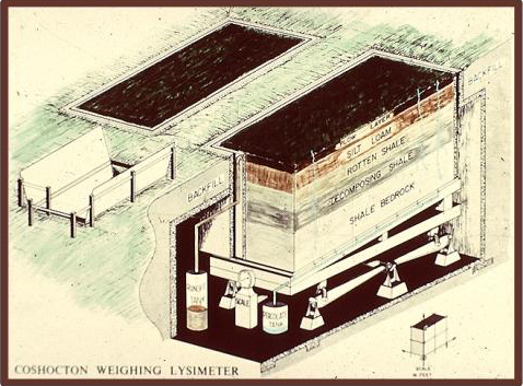Iconic models are simplified representations of real-world hydrologic systems, such as lysimeters, rainfall simulators, and experimental watersheds (Fig. 1-7). Analog models are those that base their measurements on substances different from those of the prototype, such as the flow of electrical current to represent the flow of water. Fig. 1-7  The USDA ARS Coshocton weighing lysimeter. In engineering hydrology, all formal models are mathematical in nature; hence the use of the term mathematical model to refer to all formal models. Unless specifically stated otherwise, the term "model" will be used in this book to refer to a mathematical model. The latter is by far the most widely used model type in engineering hydrology. Mathematical models can be either: (1) theoretical, (2) conceptual, or (3) empirical. A theoretical model is founded on a set of general laws; conversely, an empirical model is largely based on inferences derived from the analysis of data. A conceptual model lies somewhere in between theoretical and empirical models. In engineering hydrology, four types of mathematical models are in current use: (1) deterministic, (2) probabilistic, (3) conceptual, and (4) parametric. A deterministic model is formulated by using laws of physical, chemical, and/or biological processes, as described by differential equations. A probabilistic model, whether statistical or stochastic, is governed by laws of chance or probability. Statistical models deal with observed samples, whereas stochastic models focus on the random properties of certain hydrologic time series; for instance, daily streamflows [5]. A conceptual model is a simplified representation of the physical processes, obtained by lumping spatial and/ or temporal variations, and described in terms of either ordinary differential equations or algebraic equations. A parametric model represents hydrologic processes by means of algebraic equations that contain key parameters to be determined by empirical means. Methods of analysis in engineering hydrology can generally be classified under one of the four model types just mentioned. For instance, the kinematic wave routing technique (Chapters 4 and 9) is deterministic, being governed by a partial differential equation describing the mass and momentum balance of fluid mechanics. The Gumbel method of flood frequency analysis (Chapter 6) is probabilistic, being based on an extreme value probability law. The cascade of linear reservoirs (Chapter 10) is conceptual, seeking to simulate the complexities of catchment response by means of a series of hypothetical linear reservoirs. The rational method (Chapter 4) is parametric, with peak flow (for a given frequency) estimated on the basis of an empirically determined runoff coefficient. In principle, deterministic models mimic physical processes and should, therefore, be closest to reality. In practice, however, the inherent complexity of physical phenomena generally limits the deterministic approach to well defined cases for which a clear cause-effect relationship can be demonstrated. Probabilistic methods are used to fit measured data (i.e., statistical hydrology) and to model random components (stochastic hydrology) in cases where their presence is readily apparent. Where simplicity is desired, conceptual and parametric methods and models continue to play an important role in engineering hydrology. Hydrologic models can be either lumped or distributed. Lumped models can describe temporal variations but cannot describe spatial variations. A typical example of a lumped hydrologic model is the unit hydrograph (Chapter 5), which describes a catchment's unit response without regard to the response of individual subcatchments. Unlike lumped models, distributed models have the capability to describe both temporal and spatial variations. Distributed models are much more computationally intensive than lumped models and are, therefore, ideally suited for use with a computer. 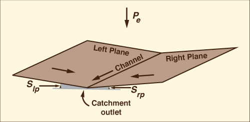A typical example of a distributed hydrologic model is an overland flow computation using routing techniques (Chapter 10) (Fig. 1-8). In this case, equations of mass and momentum (or surrogates thereof) are used to compute temporal variations of discharge and flow depth at several locations within a catchment. Fig. 1-8  Two planes-one channel overland flow configuration. Solutions to hydrologic models can be either analytical or numerical. Analytical solutions are obtained by using classical tools of applied mathematics, such as Laplace transforms, perturbation theory, and the like [3]. Numerical solutions are obtained by discretizing differential equations into algebraic equations and solving them, usually with the aid of a computer. Examples of analytical solutions are the linear models used in hydrologic systems analysis [1]. Examples of numerical solutions abound, such as those used in hydrologic routing techniques (Chapters 8, 9 and 10) and in the computer models in current use (Chapter 13). 1.6  FLOOD HYDROLOGY AND CATCHMENT SCALE [Questions]   [Problems]   [References]   •   [Top]   [Definition]   [Hydrologic Cycle]   [Catchment Budget]   [Uses]   [Approaches]   At the catchment level, surface runoff typically occurs either: (a) when rainfall intensity exceeds the abstractive capability of the catchment surface, or (b) when the soil profile is completely saturated with moisture, with infiltration being reduced to negligible amounts. Eventually, large amounts of surface runoff originating at the catchment level concentrate to produce large flow rates referred to as floods. The study of floods, their occurrences, causes, transport, and effects, is the subject of flood hydrology. In nature, rainfall varies in space and time. In engineering hydrology, rainfall can be assumed to be either: (1) constant in both space and time, (2) constant in space but varying in time, or (3) varying in both space and time. The catchment scale helps determine which one of these assumptions is justified on practical grounds. Generally, small catchments are those in which runoff can be modeled by assuming constant rainfall in both space and time. Midsize catchments are those in which runoff can modeled by assuming rainfall to be constant in space but to vary in time. Large catchments are those in which runoff can be modeled by assuming rainfall to vary in both space and time. 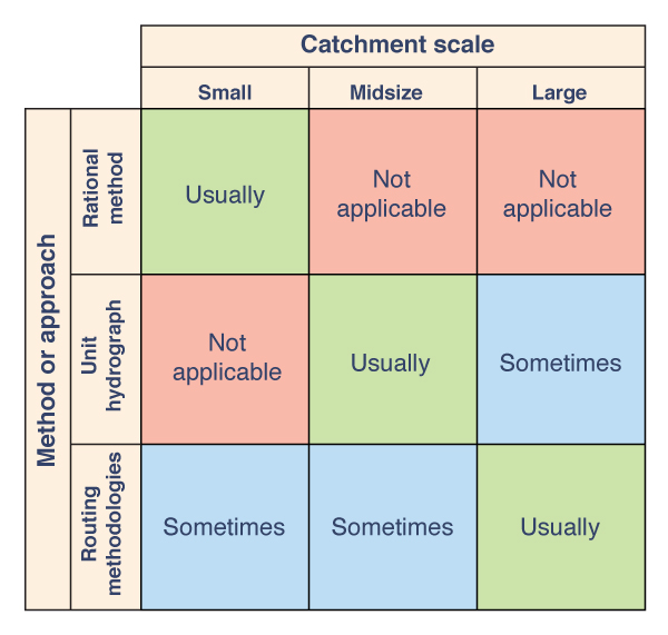In flood hydrology, small catchments are usually modeled with a simple empirical approach, such as the rational method (Chapter 4). For midsize catchments, a lumped conceptual model such as the unit hydrograph is preferred by most engineers in practice (Chapter 5). For large catchments, temporal and spatial variations of rainfall and runoff may dictate the use of a distributed modeling approach, including reservoir and stream channel routing (Chapters 8 and 9). Figure 1-9 shows a matrix depicting the relationship between catchment scale and three commonly used approaches to flood hydrology. Fig. 1-9  Relationship between catchment scale and three commonly used approaches to flood hydrology. The larger the catchment, the more likely it is to be gaged, i.e., to possess a streamflow record. Conversely, the smaller the catchment, the more unlikely it is to be gaged. This fact dictates that the probabilistic approach (Chapter 6) is primarily applicable to large catchments, particularly to those possessing a fairly long record period. For ungaged catchments or for gaged catchments with relatively short record periods, statistical techniques can be used to develop parametric models having regional applicability (Chapter 7). The subjects of catchment routing (Chapter 10) and catchment modeling (Chapter 13) span the gamut of hydrologic applications, from small to large catchments. QUESTIONS [Problems]   [References]   •   [Top]   [Definition]   [Hydrologic Cycle]   [Catchment Budget]   [Uses]   [Approaches]   [Flood and Scale]   What is the hydrologic cycle? Name the liquid-transport phases of the hydrologic cycle. Name the vapor-transport phases of the hydrologic cycle. What is a catchment? Give two examples of engineering problems (different from those mentioned in the text) where hydrologic knowledge is necessary to obtain a solution. What is material model? A formal model? What is an iconic model? An analog model? What is a deterministic model ? A lumped model? Contrast conceptual and parametric models. Contrast analytical and numerical solutions. What is a small catchment from the flood hydrology standpoint? A midsize catchment? A large catchment? PROBLEMS [References]   •   [Top]   [Definition]   [Hydrologic Cycle]   [Catchment Budget]   [Uses]   [Approaches]   [Flood and Scale]   [Questions]   During a given year, the following hydrologic data were collected for a 2500-km2 basin: total precipitation, 620 mm; total combined loss due to evaporation and evapotranspiration, 320 mm; estimated groundwater outflow (including groundwater depletion), 100 mm ; and mean surface runoff, 150 mm. What is the change in volume of water remaining in storage in the basin during the elapsed year? (Volume in hm3, i.e., millions of cubic meters). During 2012, the following hydrologic data were collected for a 85-mi2 watershed: total precipitation, 27 in.; total combined loss due to evaporation and evapotranspiration, 10 in.; estimated groundwater outflow (including groundwater depletion), 7 in.; and mean surface runoff, 9 in. What is the change in volume of water remaining in storage in the watershed during 2012? (Volume in ac-ft). During a given year, the following hydrologic data were collected for a certain 350-km2 catchment: total precipitation, 850 mm; combined evaporation and evapotranspiration, 420 mm; and surface runoff, 225 mm. Calculate the volume of infiltration (in hm3, i.e., millions of cubic meters), neglecting changes in surface water storage and groundwater effects. During a given year, the following hydrologic data were measured for a certain 60-mi2 watershed: total precipitation, 35 in.; and estimated losses due to evaporation, evapotranspiration, and infiltration, 28 in. Calculate the mean annual runoff (in ft3/s). Neglect changes in surface water storage and groundwater effects. REFERENCES •   [Top]   [Definition]   [Hydrologic Cycle]   [Catchment Budget]   [Uses]   [Approaches]   [Flood and Scale]   [Questions]   [Problems]   Agricultural Research Service, U.S. Department of Agriculture. (1973). "Linear Theory of Hydrologic Systems," Technical Bulletin No. 1468. (J.C.I. Dooge, author). Washington, D .C., October. Eagleson, P. S. (1970) . Dynamic Hydrology. New York: McGraw-Hill. Lighthill, M. J., and G. B. Whitham. (1955). On kinematic waves. I. Flood movement in long rivers. Proceedings of the Royal Society of London, Vol. A229, May, 281-316. Woolhiser, D. A., and D. L. Brakensiek. (1982). "Hydrologic Modeling of Small Watersheds," Chapter 1 in Hydrologic Modeling of Small Watersheds, edited by C. T. Haan et al. ASAE Monograph No. 5, St. Joseph, Michigan. Yevjevich, V. (1972). Stochastic Processes in Hydrology. Fort Collins, Colo.: Water Resources Publications. http://engineeringhydrology.sdsu.edu 160829