|
|
|
CHAPTER 2: HYDROLOGIC PRINCIPLES |
|
"Discharge by wells must be balanced by an increase in the recharge of the aquifer, or by a decrease in the old natural discharge, or by a loss of storage, or by a combination of these." Charles V. Theis (1940) |
|
This chapter is divided into four sections. Section 2.1 deals with precipitation, its meteorological aspects, quantitative description, spatial and temporal variations, and data sources. Section 2.2 discusses hydrologic abstractions that are important in engineering hydrology: interception, infiltration, surface storage, evaporation, and evapotranspiration. Section 2.3 defines geometric and other catchment properties relevant to hydrologic analysis. Section 2.4 deals with runoff analysis, both in a qualitative and quantitative way. The concepts presented in this chapter are of an introductory nature, intended to provide the necessary background for the more specialized study that will follow. |
2.1 PRECIPITATION
|
|
Introduction
Engineering hydrology takes a quantitative view of the hydrologic cycle. Generally, equations are used to describe the interaction between the various phases of the hydrologic cycle. As shown in Chapter 1, the following basic equation relates precipitation and surface runoff:
| Q = P - L | (2-1) |
in which Q = surface runoff, P = precipitation; and L = losses, or hydrologic abstractions. The latter term is interpreted as the summation of the various precipitation-abstracting phases of the hydrologic cycle.
Rainfall is the liquid form of precipitation; snowfall and hail are the solid forms. In common usage, the word rainfall is often used to refer to precipitation. Exceptions are the cases where a distinction between liquid and solid precipitation is warranted.
Generally, the catchment has an abstractive capability that acts to reduce total rainfall into effective rainfall. The difference between total rainfall and effective rainfall is the losses or hydrologic abstractions. The abstractive capability is a characteristic of the catchment, varying with its level of stored moisture. Hydrologic abstractions include interception, infiltration, surface storage, evaporation, and evapotranspiration. The difference between total rainfall and hydrologic abstractions is called runoff. Therefore, the concepts of effective rainfall and runoff are equivalent.
The terms in Eq. 2-1 can be expressed as rates (millimeters per hour, centimeters per hour, or inches per hour), or when integrated over time, as depths (millimeters, centimeters or inches). In this sense, a given depth of rainfall or runoff is a volume of water uniformly distributed over the catchment area.
Meteorological Aspects
The earth's atmosphere contains water vapor. The amount of water vapor may be conveniently expressed in terms of a depth of precipitable water. This is the depth of water that would be realized if all the water vapor in the air column above a given area were to condense and precipitate on that area.
There is an upper limit to the amount of water vapor in an air column. This upper limit is a function of the air temperature. The air column is considered to be saturated when it contains the maximum amount of water vapor for its temperature. Lowering the air temperature results in a reduction of the air column's capacity for water vapor. Consequently, an unsaturated air column, i.e., one that has less than the maximum amount of water vapor for its temperature, can become saturated without the actual addition of moisture if its temperature is lowered to a level at which the actual amount of water vapor will produce saturation. The temperature to which air must be cooled, at constant pressure and water vapor content, to reach saturation is called the dewpoint. Condensation usually occurs at or near saturation of the air column.
Cooling of Air Masses. Air can be cooled by many processes. However, adiabatic cooling by reduction of pressure through lifting is the only natural process by which large air masses can be cooled rapidly enough to produce appreciable precipitation. The rate and amount of precipitation are a function of the rate and amount of cooling and of the rate of moisture inflow into the air mass to replace the water vapor that is being converted into precipitation.
The lifting required for the rapid cooling of large air masses is due to four processes [72]:
- Frontal lifting,
- Orographic lifting,
- Lifting due to horizontal convergence, and
- Thermal lifting.
More than one of these processes is usually active in the lifting associated with the heavier precipitation rates and amounts.
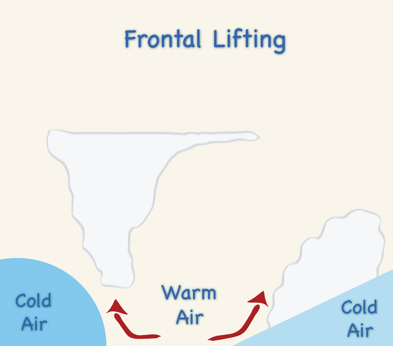
Frontal lifting takes place when relatively warm air flowing towards a colder (hence denser) air mass is forced upward, with the cold air acting as a wedge (Fig. 2-1 (a)). Cold air overtaking warmer air will produce the same result by wedging the latter aloft. The surface of separation between the two different air masses is called a frontal surface. A frontal surface always slopes upward toward the colder air mass; the intersection of the frontal surface with the ground is called a front .
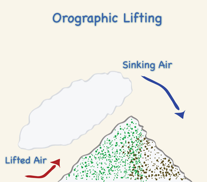
Orographic lifting occurs when air flowing toward an orographic barrier (i.e., mountain) is forced to rise in order to pass over it (Fig. 2-1 (b)). The slopes of orographic barriers are usually steeper than the steepest slopes of frontal surfaces. Consequently, air is cooled much more rapidly by orographic lifting than by frontal lifting.
|
|
|
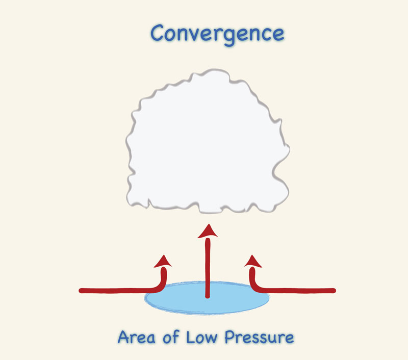
Lifting due to horizontal convergence is also important in the production of clouds and precipitation. Convergence occurs when the pressure and wind (velocity) fields act to concentrate inflow of air into a particular area, such as a low-pressure area (Fig. 2-1 (c)). If this convergence takes place in the lower layers of the atmosphere, the tendency to pile up forces the air upward, resulting in its cooling. Even when precipitation does not result from convergence alone, subsequent precipitation triggered by other processes may be more intense if convergence has occurred.
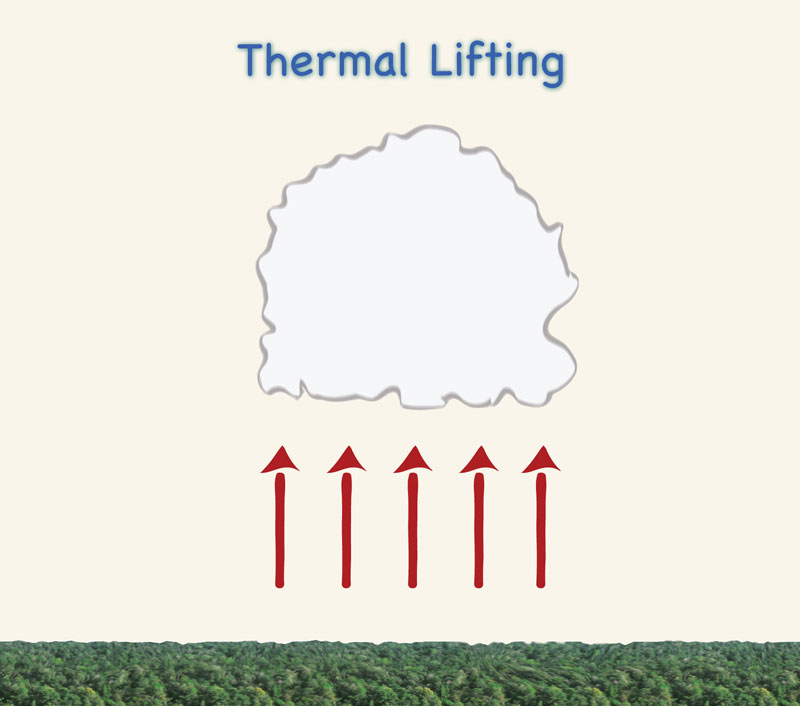
Thermal lifting is caused by local heating. As heated surface air becomes buoyant, it is forced to rise, resulting in its cooling. If the local heated air contains enough moisture and rises far enough, saturation will be reached and cumulus clouds will form (Fig. 2-1 (d)). Thermal lifting is more pronounced in the warm season. Rainfall associated with thermal lifting is likely to be scattered in geographic extent. In flat country, the greatest convective activity is over the hottest surfaces; in mountain country, it is greatest over the highest peaks and ridges.
|
|
Condensation of Water Vapor into Liquid or Solid Form. Condensation is the process by which water vapor in the atmosphere is converted into liquid droplets or, at low temperatures, into ice crystals. The results of the process are often, but not always, visible in the form of clouds, which are airborne liquid water droplets or ice crystals or a mixture of these two.
Saturation does not necessarily result in condensation. Condensation nuclei are required for the conversion of water vapor into droplets. Among the more effective condensation nuclei are certain products of combustion and salt particles from the sea. There are usually enough condensation nuclei in the air to produce condensation when the water vapor reaches saturation point.
Growth of Cloud Droplets and Ice Crystals to Precipitation Size. When air is cooled below its initial saturation, so that temperature and condensation continues to take place, liquid droplets or ice crystals tend to accumulate in the resulting cloud. The rate at which this excess liquid and solid moisture is precipitated from the cloud depends upon: (1) the speed of the upward current producing the cooling, (2) the rate of growth of the cloud droplets into raindrops heavy enough to fall through the upward current, and (3) a sufficient inflow of water vapor into the area to replace the precipitated moisture.
Water droplets in a typical cloud usually average about 0.01 mm in radius and weigh so little at an upward current of only 0.0025 m/s is sufficient to keep them from falling. Although no definite drop size can be said to mark the boundary between cloud and raindrops, a radius of 0.1 mm has been generally accepted. The radius of most raindrops reaching the ground is usually much greater than 0.1 mm and may reach 3 mm. Drops larger than this tend to break into smaller drops because the surface tension is insufficient to withstand the distortions the drop undergoes in falling through the air. Drops of 3 mm radius have a terminal velocity of about 10 m/s; therefore, an unusually strong upward current would be required to keep a drop of this size from falling.
Various theories have been advanced to explain the growth of a cloud element into a size that can precipitate. The two principal processes in the formation of precipitation are: (1) the ice crystal process, and (2) the coalescence process [29]. These two processes may operate together or separately. The ice crystal process involves the presence of ice crystals in a supercooled (cooled to below freezing) water cloud. Due to the fact that saturation vapor pressure over water is greater than that over ice, there is a vapor pressure gradient from water drops to ice crystals. This causes the ice crystals to grow at the expense of the water drops and, under favorable conditions, to attain precipitation size. The ice crystal process is operative only in supercooled water clouds, and it is most effective at about -15oC.
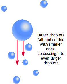
The coalescence process is based on the difference in fall velocities and consequent collisions to be expected between cloud elements of different sizes (Fig. 2-2). The rate of growth of cloud elements by coalescence depends upon the initial range of particle sizes, the size of the largest drops, the drop concentration, and the sizes of the aggregated drops. The electric field and drop charge may affect collision efficiencies and may therefore be important factors in the release of precipitation from clouds [71]. Unlike the ice crystal process, the coalescence process occurs at any temperature, lts effectiveness varying from solid to liquid particles.
Fig. 2-2 The coalescence process (cmmap.org). |
Forms of Precipitation. Precipitation occurs primarily in the form of drizzle, rain, hail, or snow (Fig. 2-3). Drizzle consists of tiny liquid water droplets, usually between 0.1 and 0.5 mm in diameter, falling at intensities rarely exceeding 1 mm/h. Rain consists of liquid water drops, mostly larger than 0.5 mm in diameter. Rainfall refers to amounts of liquid precipitation. Rainfall intensities can be classified as: light, up to 3 mm/h; moderate, from 3 to 10 mm/h; and heavy, over 10 mm/h. A rainstorm is a rainfall event lasting a clearly defined duration.
Fig. 2-3 Forms of precipitation. |
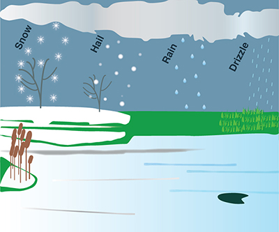
Hail is composed of solid ice stones or hailstones. Hailstones may be spheroidal, conical, or irregular in shape and may range from about 5 to over 125 mm in diameter. A hailstorm is a precipitation event in the form of hail.
Snow is composed of ice crystals, primarily in complex hexagonal form and often aggregated into snowflakes that may reach several millimeters in diameter. Snowfall is precipitation in the form of snow. A snowstorm is a snowfall event with a clearly defined duration. Snowpack is the volume of snow accumulated on the ground after one or more snowstorms. Snowmelt, or melt, is the volume of snow that has changed from solid to liquid state and is available for runoff.
Factors affecting precipitation. Table 2-1 shows the various factors affecting precipitation and their effect on: (a) moisture availability, (b) condensation, and (c) coalescence. Factors No. 1 to 7 are entirely of natural origin and, therefore, not subject to anthropogenic control. Factor No. 8 may be subject to either natural or anthropogenic control. Factor No. 9 is the only factor which is subject to anthropogenic control.
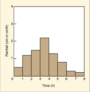
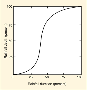
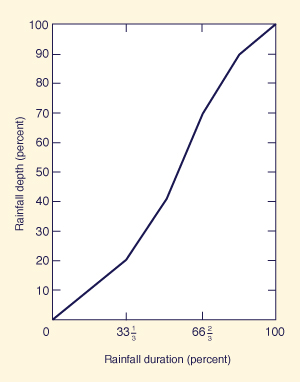
A rainfall event, or storm, describes a period of time having measurable and significant rainfall, preceded and followed by periods with no measurable rainfall. The time elapsed from start to end of the rainfall event is the rainfall duration. Typically, rainfall duration is measured in hours. However, for very small catchments it may be measured in minutes, while for very large catchments it may be measured in days. Rainfall durations of 1, 2, 3, 6, 12, and 24 h are common in hydrologic analysis and design. For small catchments, rainfall durations can be as short as 5 min. Conversely, for large river basins, durations of 2 d and longer may be applicable [78]. Rainfall depth is measured in mm, cm, or in., considered to be uniformly distributed over the catchment area. For instance, a 60-mm, 6-h rainfall event produces 60 mm of depth over a 6-h period. Rainfall depth and duration tend to vary widely, depending on geographic location, climate, microclimate, and time of the year. Other things being equal, larger rainfall depths tend to occur more infrequently than smaller rainfall depths. For design purposes, rainfall depth at a given location is related to the frequency of its occurrence. For instance, 60 mm of rainfall lasting 6 h may occur on the average once every 10 y at a certain location. However, 80 mm of rainfall lasting 6 h may occur on the average once every 25 y at the same location. Average rainfall intensity is the ratio of rainfall depth to rainfall duration. For example, a rainfall event producing 60 mm in 6 h represents an average rainfall intensity of 10 mm/h. Rainfall intensity, however, varies widely in space and time, and local or instantaneous values are likely to be very different from the spatial and temporal average. Typically, rainfall intensities are in the range 0.1-30 mm/h, but can be as large as 150 to 350 mm/h in extreme cases. Rainfall frequency refers to the average time elapsed between occurrences of two rainfall events of the same depth and duration. The actual elapsed time varies widely and can therefore be interpreted only in a statistical sense. For instance, if at a certain location a 100-mm rainfall event lasting 6 h occurs on the average once every 50 y, the 100-mm, 6-h rainfall frequency for this location would be 1 in 50 years, 1/50, or 0.02. The reciprocal of rainfall frequency is referred to as return period, or recurrence interval. In the case of the previous example, the return period corresponding to a frequency of 0.02 is 50 y. Generally, larger rainfall depths tend to be associated with longer return periods. The longer the return period, the longer the historical record needed to ascertain the statistical properties of the distribution of annual maximum rainfall. Due to the paucity of long rainfall records, extrapolations are usually necessary to estimate rainfall depths associated with long return periods. These extrapolations entail a certain measure of risk. When the risk involves human life, the concepts of rainfall frequency and return period are no longer considered adequate for design purposes. Instead, a reasonable maximization of the meteorological factors associated with extreme precipitation is used, leading to the concept of Probable Maximum Precipitation (PMP). For a given geographic location, catchment area, event duration, and time of the year, the PMP is the theoretically greatest depth of precipitation. In flood hydrology studies, the PMP is used as a basis for the calculation of the Probable Maximum Flood (PMF). For certain projects, a precipitation depth less than the PMP may be justified on economic grounds. This leads to the concept of Standard Project Storm (SPS). The SPS is taken as an appropriate percentage of the applicable PMP and is used to calculate the Standard Project Flood (SPF) (Chapter 14). Temporal and Spatial Variation of Precipitation Temporal Rainfall Distribution. Rainfall intensities for events of short duration (1 h or less) can usually be expressed as an average value, obtained by dividing rainfall depth by rainfall duration. For longer events, instantaneous values of rainfall intensity are likely to become more important, particularly for flood peak determinations. The temporal rainfall distribution depicts the variation of rainfall depth within a storm duration. It can be expressed in either discrete or continuous form. The discrete form is referred to as a hyetograph, a histogram of rainfall depth (or rainfall intensity) with time increments as abscissas and rainfall depth (or rainfall intensity) as ordinates, as shown in Fig. 2-4 (a). The continuous form is the temporal rainfall distribution, a function describing the rate of rainfall accumulation with time. Rainfall duration (abscissas) and rainfall depth (ordinates) can be expressed in percentage of total value, as shown in Fig. 2-4 (b). The dimensionless temporal rainfall distribution is used to convert a storm depth into a hyetograph, as shown in the following example.
Spatial Rainfall Distribution. Rainfall varies not only temporally but
also spatially, i.e., the same amount of rain does not fall uniformly over the entire catchment.
Isohyets
are used to depict the spatial variation of rainfall. An isohyet is a contour line showing the loci of
equal rainfall depth
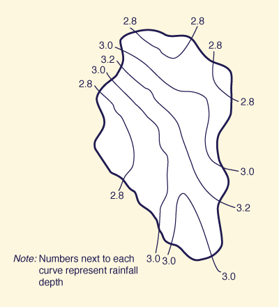
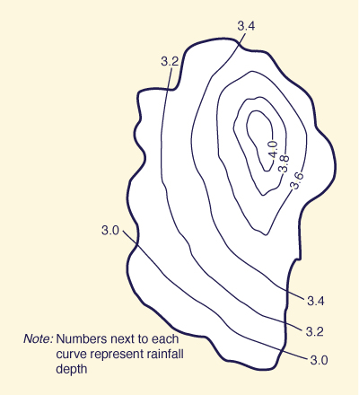
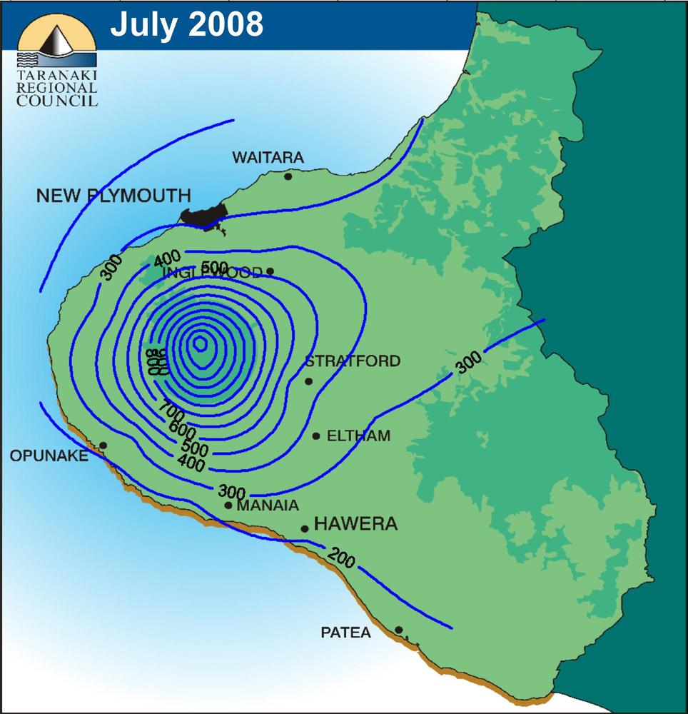
Individual storms may have a spatial distribution or pattern in the form of concentric isohyets of approximately elliptic shape. This gives rise to the term storm eye to depict the center of the storm (Fig. 2-6 (b)). In general; storm patterns are not static, moving gradually in a direction approximately parallel to that of the prevailing winds. Isohyets are also used to show spatial rainfall patterns for a given time period. Figure 2-7 shows an example of spatial rainfall distribution for the month of July 2008 in Taranaki, New Zealand.
| |||||||||||||||||||||||||||||||||||||||||||||||||||||||||||||||||||||||||||||||||||||||
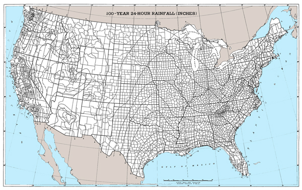
For regional rainfall mapping, isohyets are commonly referred to as isopluvials. Isopluvial maps for the United States are published by the National Weather Service [58, 59, 85-88]. These maps show contours of equal rainfall depth, applicable for a range of durations, frequencies, and geographical locations; see, for example, Fig. 2-8 for San Diego County, California, and Fig. 2-9 for the contiguous United States.
Fig. 2-8 100-yr 24-h isopluvials for San Diego County, California (0.1 in) (Source: NOAA) (Click -here- to display). |
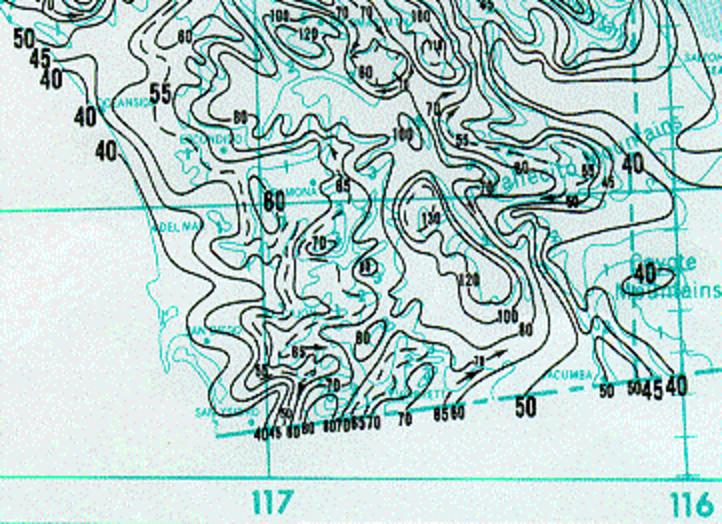
Fig. 2-9 100-yr 24-h isopluvials for the contiguous United States (in.) (NOAA) (Click -here- to display). |
For large catchments, highly intensive storms (thunderstorms) may cover only a fraction of the whole basin, yet they may lead to severe flooding in localized areas. The role of thunderstorms in determining the flood potential of large basins is usually assessed on an individual basis.
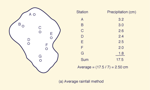
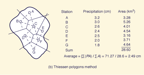
Average Precipitation Over an Area. A precipitation (or rainfall) amount is measured with rain gages. During a given storm, it is likely that the depth measured by two or more rain gages of the same type will not be the same. In hydrologic analysis, it is often necessary to determine a spatial average of the rainfall depth over the catchment. This is accomplished by either of the following methods:
- Average rainfall,
- Thiessen polygons, and
- Isohyetal curves.
In the average rainfall method, the rainfall depths measured by the rain gages located within the catchment are tabulated. These rainfall depths are then averaged to find the average precipitation over the catchment, as shown in Fig. 2-10 (a).
Fig. 2-10 (a) Average rainfall method (Click -here- to display). |
In the Thiessen polygons method, the locations of the rain gages are plotted on a scale map of the catchment and surrounding area. The locations (stations) are joined with straight lines in order to form a pattern of triangles, preferably with sides of approximately equal length. Perpendicular bisectors to the sides of these triangles are drawn to enclose each station within a polygon called a Thiessen polygon, circumscribing an area of influence, as shown in Fig. 2-10 (b). The average precipitation over the catchment is calculated by weighing each station's rainfall depth in proportion to its area of influence.
Fig. 2-10 (b) Thiessen polygons method (Click -here- to display). |
In the isohyetal method, the locations of the rain gages are plotted on a scale map of the catchment and surrounding area. Each station's rainfall depth is used to draw isohyets throughout the catchment in a manner similar to that used in the preparation of topographic contour maps. The mid-distance between two adjacent isohyets is used to delineate the area of influence of each isohyet, as shown in Fig. 2-10 (c). The average precipitation over the catchment is calculated by weighing each isohyetal increment in proportion to its area of influence.
Fig. 2-10 (c) Isohyetal method (Click -here- to display). |
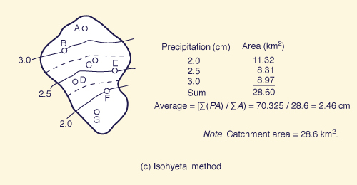
The isohyetal method is regarded as more accurate than either the Thiessen polygons or average rainfall methods. This is particularly the case when averaging precipitation over catchments where orographic effects have a significant influence on the local storm pattern. The Thiessen polygons method is generally more accurate than the average rainfall method. The increase in accuracy is likely to be more marked when averaging precipitation over catchments with widely varying rainfall depths or large differences in areas of influence.
Storm Analysis
Storm Depth and Duration. Storm depth and duration are directly related, storm depth increasing with duration. An equation relating storm depth and duration is:
| h = c t n | (2-2) |
in which h = storm depth, in centimeters; t = storm duration, in hours; c = a coefficient; and n = an exponent (a positive real number less than 1). Typically, n varies between 0.2 and 0.5, indicating that storm depth increases at a lesser rate than storm duration. By analyzing storm data on a regional or local basis, Eq. 2-2 can be used to predict storm depth as a function of storm duration. The applicability of such an equation, however, is limited to the regional or local conditions for which it was derived.
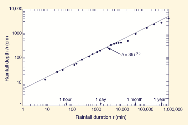
Equation 2-2 can also be used to study the characteristics of extreme rainfall events. A logarithmic plot of depth-duration data for the world's greatest observed rainfall events (Table 2-2) results in the following enveloping line:
| h = 39 t 0.5 | (2-3) |
in which h = rainfall depth, in centimeters, and t = rainfall duration, in hours. The data of Table 2-2 are plotted in Fig. 2-11, including the enveloping line, Eq. 2-3.
| ||||||||||||||||||||||||||||||||||||||||||||||||||||||||||||||||||||||||||||||||||||||||||||||||||||
Fig. 2-11 Depth-duration data for the world's greatest observed rainfall events. |
Storm Intensity and Duration. Storm intensity and duration are inversely related. From Eq. 2-2, an equation linking storm intensity and duration, can be obtained by differentiating rainfall depth with respect to duration, to yield:
|
dh ______ = i = c n t n -1 dt | (2-4) |
in which i = storm intensity. Simplifying,
|
a i = ______ t m | (2-5) |
in which a = cn, and m = 1 - n. Since n is less than 1, it follows that m is also less than 1.
Another intensity-duration model is the following:
|
a i = _________ t + b | (2-6) |
in which a and b are constants to be determined by regression analysis (Chapter 7).
A general intensity-duration model combining the features of Eqs. 2-5 and 2-6 is:
|
a i = _____________ ( t + b ) m | (2-7) |
For b = 0, Eq. 2-7 reduces to Eq. 2-5; for m = 1, Eq. 2-7 reduces to Eq. 2-6.
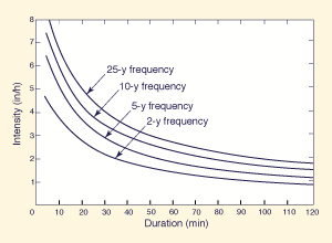
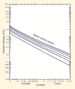
Intensity-Duration-Frequency. For small catchments it is often necessary to determine several intensity-duration curves, each for a different frequency or return period. A set of intensity-duration-frequency curves is referred to as IDF curves, with duration plotted in the abscissas, intensity in the ordinates, and frequency (or alternatively, return period) as curve parameter. Either arithmetic (Fig. 2-12 (a)) or logarithmic (Fig. 2-12 (b)) scales are used in the construction of IDF curves. Such curves are developed by government agencies for use in urban storm-drainage design and other applications (Chapter 4).
A formula for IDF curve can be obtained by assuming that the constant a in Eqs. 2-5 through 2- 7 is related to return period T as follows:
| a = k T n | (2-8) |
in which k = a coefficient; T = return period; and n = an exponent (not related to that of Eq. 2-2). This leads to
|
k T n i = _____________ ( t + b ) m | (2-9) |
The values of k, b, m, and n are evaluated from measured data or local experience.
|
|
Storm Depth and Catchment Area. Generally, the greater the catchment area, the smaller the spatially averaged storm depth. This variation of storm depth with catchment area has led to the concept of point depth, defined as the storm depth associated with a given point area. A point area is the smallest area below which the variation of storm depth with catchment area can be assumed to be negligible. In the United States, the point area is usually taken as 25 km2 (10 mi2).
The point depth applies for all areas less than the point area. For areas greater than the point area, a reduction in point depth is necessary to account for the decrease of storm depth with catchment area. This depth reduction is accomplished with a depth-area reduction chart, a function relating catchment area (abscissas) to point depth percentage (ordinates). Storm duration is usually a curve parameter in a depth-area reduction chart.
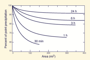
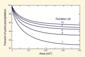
Generalized depth-area reduction charts applicable to the contiguous United States, for areas up to 1000 km2 (400 mi2) and durations from 30 min to 10 d have been published by the National Weather Service (Figs. 2-13 (a) and (b)). Regional and locally derived depth-area reduction charts may differ from these generalized charts (see Section 14.1).
|
|
Depth-Duration-Frequency. For midsize catchments, hydrologic analysis shifts its focus to rainfall depth. Isopluvial maps depicting storm depths, applicable for a range of durations, frequencies and catchment areas, are available for the entire United State [58, 59, 85-88]. These maps show point depth values and are therefore subject to depth-area reduction by the use of an appropriate chart.
Depth-Area-Duration. Another way of describing the relation between storm depth, duration and catchment area is the technique known as depth-area-duration (DAD) analysis. This technique is basically an alternate way of portraying the reduction of storm depth with area, with duration as a third variable.
To construct a DAD chart, a storm having a single major center (storm eye) is identified.
Isohyetal maps showing maximum storm depths for each of several typical durations (6-h, 12-h, 24-h, etc.) are prepared.
For each map, the isohyets are taken as boundaries
circumscribing individual areas. For each map and each individual area, a spatially
averaged rainfall depth is calculated by dividing the total rainfall volume by the
individual area. This procedure provides DAD data sets used to construct a chart showing
depth versus area, with duration as a curve parameter (Fig. 2-14).
Fig. 2-14 A depth-area duration curve. |
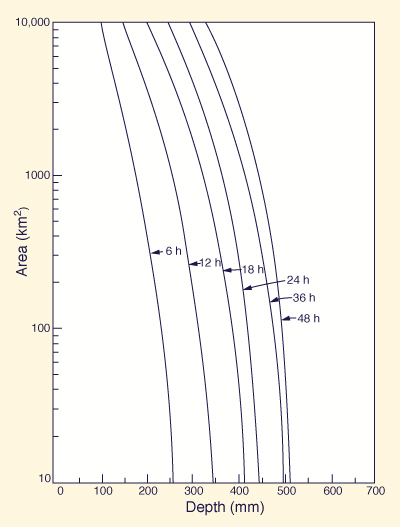
DAD analysis can also be used to study regional rainfall characteristics. Table 2-3 shows maximum DAD data for the United States, based on four extreme events. The data confirm that storm depth increases with duration and decreases with catchment area.
| |||||||||||||||||||||||||||||||||||||||||||||||||||||||||||||||||||||||||||||||||||||||
Probable Maximum Precipitation. For large projects, storm analysis using depth-duration-frequency data is not sufficient to eliminate the likelihood of failure. In such cases, the concept of PMP is used instead. In the United States, PMP estimates are developed following guidelines included in the HM NOAA Hydrometeorological Reports) serie [33-44] and related publications [84-87]. These reports contain methodologies and maps for the estimation of PMP for a given geographic location, range of durations and catchment sizes, and time of the year (Chapter 14).
Geographic and Seasonal Variations of Precipitation
Precipitation varies not only temporally and spatially but also seasonally, annually, and with geographic location and climate. Mean annual precipitation, the total amount of precipitation that accumulates in one year, on the average, at a given location, is used for classify climates (in terms of precipitation) into eight classes [11]:
- Superarid: Less than 100 mm
- Hyperarid: 100 - 200 mm
- Arid: 200 - 400 mm
- Semiarid: 400 - 800 mm
- Subhumid: 800 - 1600 mm
- Humid: 1600 - 3200 mm
- Hyperhumid: 3200 - 6400 mm.
- Superhumid: More than 6400 mm.
The seasonality of precipitation is assessed with the precipitation seasonality index: the ratio of accumulated precipitation for the three wettest consecutive months to that for the three driest consecutive months, in an average year. This index is used to classify climates into four classes [11]:
- Nonseasonal: 1.0 - 1.6
- Weakly seasonal: 1.6 - 2.5
- Moderately seasonal: 2.5 - 10
- Strongly seasonal: Greater than 10.
In general, arid and semiarid climates are associated with moderately seasonal regimes; conversely, subhumid and humid climates are associated with weakly seasonal or nonseasonal regimes. However, there are some exceptions; for instance, the monsoon-type climates which prevail in some parts of the world, which tend to be both humid and seasonal.
Precipitation Data Sources and Interpretation
Precipitation data are obtained by measurement using rain gages (Chapter 3). The National Climatic Data Center (NCDC), Asheville, North Carolina, publishes precipitation data for about 8000 stations in the United States. A large number of additional gages are operated by other federal, state, and local agencies, and by individuals. U.S. federal agencies collecting precipitation data on a regular basis include the National Weather Service (NWS), the Army Corps of Engineers, the Natural Resources Conservation Service (formerly Soil Conservation Service), the Forest Service, the Bureau of Reclamation, and the Tennessee Valley Authority.
NCDC assembles precipitation data using hourly, daily, monthly, and yearly intervals. Hourly precipitation data and maximum 15-minute duration amounts are found in Hourly Precipitation Data. Daily and monthly precipitation data are found in Climatological Data. Monthly and annual precipitation data for about 250 major U.S. cities, including hourly rates, are found in Local Climatological Data.
Regional precipitation-frequency atlases (U.S. Weather Bureau No. 40 [86], NOAA Technical Memorandum NWS Hydro-35 [59] and Precipitation Frequency Atlas of the Western United States [58]) are available. NCDC Monthly and seasonal precipitation maps are found in Weekly Weather and Crop Bulletin, available from NOAA/USDA Joint Agricultural Weather Facility, in the USDA South Building, Washington, D.C. Additional sources of precipitation data are given in Annotated Bibliography of NOAA Publications of Hydrometeorological Interest, updated at regular intervals by NWS, and in Selective Guide to Climatic Data Sources, updated at regular intervals by NCDC.
Precipitation and other relevant climatological data are now accessible online through NCDC's website at http://www.ncdc.noaa.gov. Clicking on On-line Data Access provides access to a host of on-line services, including U.S. monthly precipitation for NWS and Cooperative sites, and the On-line Access and Service Information System (OASIS), which includes hourly and 15-minute precipitation data.
Filling In Missing Records. Incomplete records of rainfall are sometimes possible due to operator error or equipment malfunction. In this case, it is often necessary to estimate the missing record. Assume that a certain station X has a missing record. A procedure to fill in the missing record is to identify three index stations (A, B, and C) having complete records, located as close to and as evenly spaced around station X as possible. The mean annual rainfall for each of the stations X, A, B, and C is evaluated. If the mean annual rainfall at each of the index stations A, B, or C is within 10 percent of that of station X, a simple arithmetic average of the rainfall values at the index stations provides the missing value at station X.
If the mean annual rainfall at any of the index stations differs by more than 10% from that of station X, the normal ratio method is used [55]. In this method, the missing precipitation value at station X is the following:
|
NX NX NX PX = (1/3) [ _____ PA + _____ PB + _____ PC ] NA NB NC | (2-10) |
in which P = precipitation, N = mean annual rainfall, and the subscripts X, A, B, and C refer to the respective stations.
An alternate method for filling in missing precipitation data has been developed by the National Weather Service [49]. The method requires data for four index stations A, B, C, and D, each located closest to the station X of interest, and in each of four quadrants delimited by north-south and east-west lines drawn through station X (Fig. 2-15). The estimated precipitation value at station X is the weighted average of the values at the four index stations. For each index station, the applicable weight is the reciprocal of the square of its distance L to station X.
Fig. 2-15 Position of station X and index stations A, B, C, and D. |
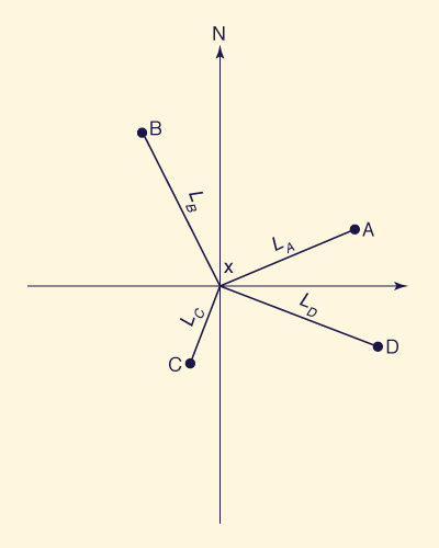
The procedure is described by the following formula:
|
4 Σ ( Pi / Li 2 ) i = 1 PX = _____________________ 4 Σ ( 1 / Li 2 ) i = 1 | (2-11) |
in which P = precipitation; L = distance between index stations and station X; and i refers to each one of the index stations A, B, C, and D.
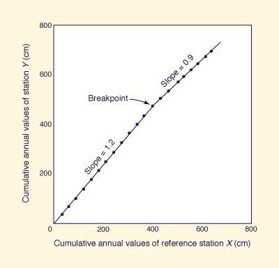
Double-mass Analysis. Changes in the location or exposure of a rain gage may have a significant effect on the amount of precipitation it measures, leading to inconsistent data (data of different nature within the same record).
The consistency of a rainfall record is tested with double-mass analysis. This method
compares the cumulative annual (or, alternatively, seasonal) values of station Y with
those of a reference station X. The reference station is usually the mean of several
neighboring stations. The cumulative pairs (double-mass values) are plotted in an x-y
arithmetic coordinate system, and the plot is examined for trend changes. If the plot is
essentially linear, the record at station Y is consistent. If the plot shows a break in slope,
the record at station Y is inconsistent and should be corrected. The correction is
performed by adjusting the records prior to the break to reflect the new state (after the
break). To accomplish this, the rainfall records prior to the break are multiplied by the
ratio of slopes after and before the break (Fig. 2-16).
Fig. 2-16 Double-mass analysis. |
2.2 HYDROLOGIC ABSTRACTIONS
|
|
Hydrologic abstractions are the processes acting to reduce total precipitation into effective precipitation. Effective precipitation eventually produces surface runoff. The difference between total and effective precipitation is the depth abstracted by the catchment.
The processes by which precipitation is abstracted by the catchment are many. Those important in engineering hydrology are the following:
- Interception,
- Infiltration,
- Surface or depression storage,
- Evaporation, and
- Evapotranspiration.
Interception
Interception is the process by which precipitation is abstracted by vegetation or other forms of surface cover, including, in certain cases, cultural features of the landscape. Interception loss is the fraction of precipitation that is retained by the vegetative cover. The intercepted amount is either returned to the atmosphere through evaporation, or go on to constitute throughfall, that part of precipitation which reaches the ground by first passing through the vegetative cover. Interception losses are a function of:
- Storm character, including intensity, depth, and duration,
- The type, species, age, and density of vegetative cover, and
- The time of the year, or season.
Interception is usually the first abstractive process to act during a storm. Light storms are substantially abstracted by the interception process. Light storms occur frequently and therefore constitute the majority of the storms. The interception loss accumulated in one year, primarily from light storms, amounts to about 25 percent of the average annual precipitation.
For moderate storms, interception losses are apt to vary widely, being greater during the growing season and smaller at other times of the year. Studies have shown that interception values are likely to vary from 7 to 36 percent of total precipitation during the growing season, and from 3 to 22 percent during the remainder of the year [12].
For heavy storms, interception losses usually amount to a small fraction of the total rainfall. For long-duration or infrequent storms, the effect of interception on the overall process of abstraction is likely to be small. In certain cases, particularly for flood hydrology studies, the neglect of interception is generally justified on practical grounds.
The interception loss comprises two distinct elements [25] The first is the interception storage, i.e., the depth (or volume) retained in the foliage against the forces of wind and gravity. The second is the evaporation loss from the foliage surface, which takes place throughout the duration of the storm. The combination of these two processes leads to the following formula for estimating interception loss [12].
|
L = S + K E t | (2-12) |
in which L = interception loss, in millimeters; S = interception storage depth in millimeters, usually varying from 0.25 to 1.25 mm; K = ratio of evaporating foliage surface to its horizontal projection; E = evaporation rate in millimeters per hour; and t = storm duration, in hours.
Infiltration
Infiltration is the process by which precipitation is abstracted by seeping into the soil below the land surface. Once below the ground surface, the abstracted water moves either laterally, as interflow, into lakes, streams, and rivers, or vertically, by percolation, into aquifers. The water that reaches lakes either evaporates or drains as lake overflow into surface streams. The water that reaches streams and rivers moves relatively rapidly toward the oceans as surface flow. The water held in aquifers moves slowly as groundwater flow, eventually flowing into a stream or reaching the ocean directly, bypassing the surface waters entirely.
Infiltration is a complex process. It is described by either an instantaneous or an average infiltration rate, both measured in millimeters per hour, or inches per hour. The total infiltration depth is obtained by integrating the instantaneous infiltration rate over the storm duration. The average infiltration rate is obtained by dividing the total infiltration depth by the storm duration.
Infiltration rates vary widely, depending on:
- The condition of the land surface, including compaction and surface crusting,
- The type and density of vegetative cover, and associated root structure,
- The physical properties of the soil, including structure, grain size, and gradation,
- The storm character, i.e., intensity, depth, and duration,
- The water temperature, and
- The water quality, including chemical constituents and other impurities.
Infiltration Formulas. For a given storm, infiltration rates tend to vary in time. The initial infiltration rate is the rate prevailing at the beginning of the storm. This rate is likely to be the maximum rate for the given storm, gradually decreasing as the storm progresses in time. For storms of long duration, the infiltration rate eventually reaches a constant value, referred to as final (or equilibrium) infiltration rate. This process led Horton [27] to describe the variation of infiltration rate with time using the following formula:
| f = fc + ( fo - fc ) e-k t | (2-13) |
in which f = instantaneous infiltration rate; fo = initial infiltration rate;
fc = final infiltration rate; k = an exponential decay
constant; and t = time, in hours.
The units of k are h-1.
For t = 0, f = fo; and for t = ∞, f
= fc (see Fig. 2-17).
Fig. 2-17 Horton's infiltration formula. |
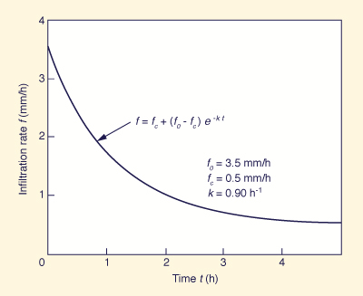
Equation 2-13 has three parameters: (1) initial infiltration rate; (2) final infiltration rate; and (3) the k value describing the rate of decay of the difference between initial and final infiltration rates. Field measurements are necessary in order to determine appropriate values of these parameters. A plot of infiltration rate versus time enables the estimation of the final rate. With a knowledge of the final rate fc , two sets of f and t are obtained from the plot and used, together with Eq. 2-13, to solve simultaneously for fo and k.
Integrating Eq. 2-13 between t = 0 and t = ∞, leads to:
|
fo - fc F = _________ k | (2-14) |
in which F = the total infiltration depth above the f = fc line. Equation 2-14 enables the calculation of the total infiltration depth, assuming that the storm lasts long enough for the equilibrium rate to be attained.
Example 2-2.
Assuming fo = 10 mm/h, fc = 5 mm/h, and k = 0.95 h-1,
calculate the total infiltration depth for a storm lasting 6 h.
After 6 h, the difference between instantaneous and
final rates is negligible. Therefore, the total infiltration depth is: (10 mm/h - 5 mm/h)/ 0.95 h-1 + (5 mm/h × 6 h)
= 35.26 mm. |
Typical infiltration rates at the end of 1 h (f1) are shown in Table 2-4. Generally, these values are reasonable approximations of final (i.e., equilibrium) infiltration rates.
| |||||||||||||||
More recent developments in infiltration theory have sought to improve on the Horton model. Philip [66] has proposed the following model:
| f = (l/2 ) s t -1/2 + A | (2-15) |
in which f = instantaneous infiltration rate; s = an empirical parameter related to the rate of penetration of the wetting front (the wetting surface characterized by a very high potential gradient); A = an infiltration value that is close to the value of saturated hydraulic conductivity at the surface; and t = time.
In Eq. 2-15, for t = 0, f = ∞; and for t = ∞, f = A. In practice, the initial infiltration rate has a finite value. In spite of this limitation, the Philip formula seems to be a good fit to experimental data. Integration of the Philip equation leads to
| F = s t 1/2 + A t | (2-16) |
in which F = total depth of infiltration.
An infiltration model with a sound theoretical basis is the Green and Ampt formula [21]. This equation describes infiltration rate under ponded water conditions as follows:
|
H + Pf f = K ( 1 + __________ ) Zf | (2-17) |
in which f = infiltration rate in millimeters per hour; K = saturated hydraulic conductivity in millimeters per hour; H = depth of ponded water in millimeters; Pf = capillary pressure at the wetting front in millimeters; and Zf = vertical depth of saturated zone in millimeters. In practice, however, it may be difficult to measure some of the terms of this equation. Recent progress has been achieved by groupe terms in Eq. 2-17 into predictable parameters linked to the physical processes [48].
Infiltration Indexes. Practical evaluations of infiltration have been hampered by its spatial and temporal variability. This has led to the use of infiltration indexes, which model the infiltration process in an approximate yet practical way.
Infiltration indexes assume that infiltration rate is constant throughout the storm duration. This assumption tends to underestimate the higher initial rate of infiltration while overestimating the lower final rate. For this reason, infiltration indexes are best suited for applications involving either long-duration storms or catchments with high initial soil moisture content. Under such conditions, the neglect of the variation of infiltration rate with time is generally justified on practical grounds.
For moderate storms, the use of infiltration indexes is largely an empirical procedure, with attention being focused on matching the prevailing soil moisture condition and storm duration in order to effect a proper balance of rainfall and runoff amounts.
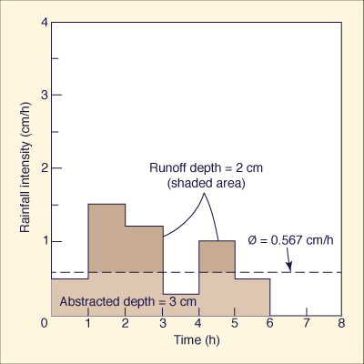
In practice, the most commonly used infiltration index is the φ-index, defined as the (constant) infiltration rate to be subtracted from the prevailing rainfall rate in order to obtain the runoff volume that actually occurred [13]. The computation of the φ-index requires a storm pattern, i.e., a plot of rainfall intensity versus time, and a measured runoff volume (or depth). The computation involves a trial-and-error procedure.
|
Example 2-3.
The runoff depth has been estimated at 2 cm. Calculate the φ-index.
From the rainfall distribution, the total rainfall is 5 cm. Therefore, the depth
abstracted by infiltration is:
[ (1.5 - φ) × 1 ] + [ (1.2 - φ) × 1 ] + [ (1.0 - φ) × 1 ] = 2 cm
From Eq. 2-18, solving for φ gives: φ = 0.567 cm/h, verifying that the assumed range
for was correct. Had the assumed range been wrong, the calculated φ-value would have been
out of that range. In Fig. 2-18, the 2 cm of runoff are above the φ-index line; the 3 cm
of abstracted rainfall are below the φ-index line. |
Fig. 2-18 Calculation of φ-index: Example 2-3. |
Another widely used infiltration index is the W-index [13], which, unlike the φ-index, takes explicit account of interception loss and depth of surface storage. The formula for the W-index is the following:
|
P - Q - S W = _____________ tf | (2-18) |
in which W = W-index, in millimeters per hour; P = rainfall depth, in millimeters; Q = runoff depth, in millimeters; S = the sum of interception loss and depth of surface storage, in millimeters; and tf = the total time (hours) during which rainfall intensity is greater than W.
The Wmin index is the W-index calculated for extremely wet conditions. It is derived using data from the last of a series of storms and is used in estimating maximum flood potential. In this sense, the Wmin index approaches a spatially averaged value of the final infiltration rate. For such extreme conditions, the values of Wmin and φ are almost identical.
Infiltration Rates Derived from Rainfall-Runoff Data. Inflltration formulas depict the variation of infiltration rates with time. Infiltration rates, however, vary not only temporally but also spatially. Unless the field measurements and related parameter estimation are fairly good representations of the spatial variability, the rates calculated by infiltration formulas are likely to be different from reality.
This difficulty is circumvented by calculating infiltration rates indirectly, from concurrent rainfall-runoff measurements. Such a calculation provides a temporal and spatial average of infiltration rate, amounting to a φ-index, with its associated advantages and disadvantages.
Infiltration and Catchment Size. For midsize and large catchments, the natural variability of infiltration rates makes it necessary to resort to the evaluation of total infiltration depth. In practice, total infiltration depths are derived from rainfall-runoff analysis. However, for each data set, the calculation is highly dependent on the level of soil moisture antecedent to the storm. The catchment moisture level is referred to as the antecedent moisture condition, or AMC (Chapter 5). Initial infiltration rates and, consequently, total infiltration depths are a function of prevailing antecedent moisture condition.
Surface or Depression Storage
Surface (or depression) storage is the process by which precipitation is abstracted by being retained in puddles, ditches, and other natural or artificial depressions of the land surface. Water held in depressions either evaporates or eventually contributes to soil moisture by infiltration. The spatial variability of storage in surface depressions precludes its precise calculation.
Intuitively, the milder the catchment's relief, the greater the effect of depression storage. Field data reported by Viessman [82] showed conclusively that depression storage is inversely related to catchment slope. Usually, an equivalent depth of depression storage can be estimated based on experience. For instance, Hicks [23] has used depression storage depths of 5.0, 3.75, and 2.5 mm for sand, loam, and clay, respectively. Tholin and Keife [77] have used values of 6.25 mm in pervious urban areas and 1.5 mm for paved areas. Where accurate estimations are difficult, depression storage amounts can be lumped together with other more tractable hydrologic abstractions such as interception or infiltration.
An alternate way of accounting for depression storage is the use of a peak-flow correction factor, as in the NRCS TR-55 graphical method (Section 5.3).
Typically, the effect of depression storage varies in time and, consequently, with storm duration. At the beginning of a storm, depression storage usually plays an active role in abstracting precipitation amounts. As time progresses, depression storage volumes are eventually filled, with any additional water going on to constitute runoff. This has led to the following conceptual model of depression storage:
| Vs = Sd ( 1 - e - k Pe ) | (2-19) |
in which Vs = equivalent depth of depression storage, in millimeters; Pe = precipitation excess, defined as total precipitation depth minus interception loss minus total infiltration depth; Sd = depression storage capacity, in millimeters; and k = a constant.
Linsley et al. [53] have suggested that values of Sd for most catchments are in the range of 10-50 mm. The value of the constant k is estimated by assuming that for very small values of precipitation excess (Pe ≅ 0), essentially all the precipitation goes into depression storage (dVs /dPe = 1). This leads to k = 1/Sd.
Evaporation
Evaporation is the process by which water accumulated on the land surface (including that held in surface depressions and water bodies such as lakes and reservoirs) is converted into vapor state and returned to the atmosphere. Evaporation occurs at the evaporating surface, the contact between water body and overlying air. At the evaporating surface, there is a continuous exchange of liquid water molecules into water vapor and vice versa. In engineering hydrology, evaporation refers to the net rate of water transfer (loss) into vapor state.
Evaporation is expressed as an evaporation rate in millimeters per day (mm/d), centimeters per day (cm/d), or inches per day (in./d). Evaporation rate is a function of several meteorological and environmental factors. Those important from an engineering hydrology standpoint are:
- Net solar radiation,
- Saturation vapor pressure,
- Vapor pressure of the air,
- Air and water surface temperatures,
- Wind velocity, and
- Atmospheric pressure.
Evaporation rates are significantly affected by climate. Studies have shown that evaporation rates
are high in arid and semiarid regions and low in humid regions. For instance, mean annual lake evaporation in
the United States varies from 20 in. (508 mm) in the Northeast (Maine) and Northwest (Washington state) corners,
to more than
80 in.
(2184 mm) in the Southwestern desert (California and Arizona) (Fig. 2-19) [18].
Fig. 2-19 Mean annual lake evaporation in the contiguous United States (NOAA). |

The effect of climate on evaporation has a substantial impact on water resources development. The planning and design of storage reservoirs in arid/semiarid regions requires a detailed evaluation of the potential for reservoir evaporation. These calculations determine to a large extent the feasibility of building surface water storage projects on regions subject to high evaporation rates.
Unlike other phases of the hydrologic cycle, lake evaporation cannot be measured directly. Therefore, several approaches have been developed to calculate evaporation. These vary in nature and are based on either: (1) a water budget, (2) an energy budget, or (3) a mass-transfer methodology.
Water Budget Method for Determining Reservoir Evaporation. The water budget method assumes that all relevant water-transport phases can be evaluated for a time period Δt, and expressed in terms of volumes. Reservoir or lake evaporation is calculated as follows:
|
E = P + Q - O - I - ΔS | (2-20) |
in which E = volume evaporated from the reservoir, P = precipitation faIling directly onto the reservoir, Q = surface runoff inflow into the reservoir, O = outflow from the reservoir, I = net volume infiltrated from the reservoir into the ground, and ΔS = change in stored volume. All terms in Eq. 2-20 refer to a time period Δt, usually taken as 1 week or greater.
Most terms in Eq. 2-20 can be evaluated directly. Precipitation is readily measured, and inflow and outflow can be obtained by integrating the flow records. The change in stored volume is determined by means of water stage recorders. Net infiltration, however, can be evaluated only indirectly, either by measuring soil permeability or monitoring changes in groundwater level in nearby wells. The difficulty in measuring net infiltration generally limits the water budget method to areas with little or no net infiltration. In spite of this limitation, the water budget method has been found to work reliably under certain idealized conditions. Water budget studies from Lake Hefner, Oklahoma, show that the method can provide evaporation volumes within a 10 percent accuracy about two-thirds of the time [81]. Conditions at Lake Hefner, however, were highly selective, and lesser accuracy is to be expected under more typical circumstances.
Energy Budget Method for Determining Reservoir Evaporation. During evaporation, significant energy exchanges occur at the evaporating surface. A balance of these energy exchanges leads to the energy budget method of calculating reservoir evaporation. The amount of heat required to convert one gram of water into vapor, i.e., the heat of vaporization, varies with temperature. For instance, at 20°C the heat of vaporization is 586 calories (Table A-1, Appendix A). To maintain the temperature of the evaporating surface, large quantities of heat must be supplied by radiation, by heat transfer from the atmosphere, and from energy stored in the water body.
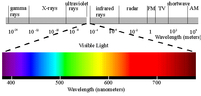
Radiation is the emission
of energy in the form of electromagnetic waves from all bodies above 0°K. Solar radiation
received on the Earth's surface is a major component of the energy balance. Solar
radiation reaches the outer surface of the atmosphere at a nearly constant flux of
about 1.95 cal/cm2/min, or langleys/min (1 langley = 1 cal/cm2), measured
perpendicular to the incident radiation. Nearly all this radiation is of wavelengths
in the range
Fig. 2-20 Range of visible light within the electromagnetic spectrum. |
In passage through the atmosphere, solar radiation changes its flux and spectral composition. Some of it is reflected back to space, and some of it is absorbed and scattered by the atmosphere. The fraction of the original solar radiation flux that reaches the Earth's surface is called direct solar radiation. The fraction of the radiation reflected and scattered by the atmosphere that reaches the ground is called sky radiation. The sum of direct solar radiation and sky radiation is called global radiation.
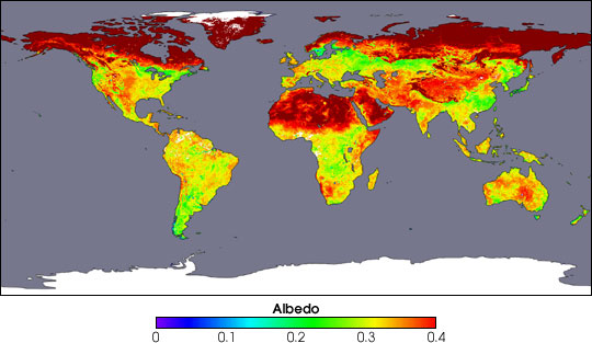
Albedo is the
reflectivity coefficient of a surface toward shortwave radiation. This coefficient varies
with color, roughness, and inclination of the surface. Its value is
| |||||||||||||||||||||||
Fig. 2-21 Global distribution of albedo (NASA). |
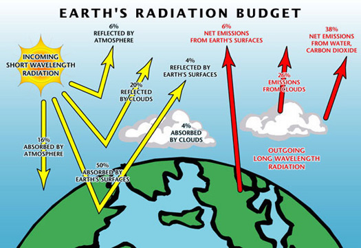
In addition to the shortwave radiation balance, there is also a longwave radiation
balance. The Earth's surface emits radiation, part of which is absorbed and reflected back
by the atmosphere. The difference between outgoing and incoming fluxes is called longwave
radiation loss. During the day, longwave radiation may be a small fraction of the total radiation
balance, but at night, in the absence of solar radiation, longwave radiation dominates the
radiation balance. Net radiation is equal to the net shortwave (solar) radiation minus the longwave (terrestrial) radiation toss (Fig. 2-22).
Fig. 2-22 The Earth's radiation budget (NASA). |
In the energy budget method, the incoming energy can be expressed as
|
Qi = Qs ( 1 - A ) - Qb + Qa | (2-21) |
in which Qi = incoming energy; Qs = global radiation (shortwave radiation from sun and sky); A = albedo; Qb = longwave radiation loss by water body; and Qa = net energy advected into the water body by streams, rain, and snow.
The energy expenditure, which must balance the incoming energy, is expressed as follows:
|
Qo = Qh + Qe + Qt | (2-22) |
in which Qo = energy expenditure; Qh = sensible heat transfer from water body to the atmosphere by convection and conduction; Qe = energy expended in the evaporation process; and Qt = increase in energy stored in the water body. The value of Qe is negative when condensation is taking place. All terms in Eqs. 2-21 and 2-22 are given in calories per square centimeter per day. The energy used in evaporation Qe (cal/cm2/day) is converted into equivalent evaporation rate E (cm/day) by the following formula:
|
Qe = ρ H E | (2-23) |
in which ρ = density of water in grams per cubic centimeter (g/cm3); H = heat of vaporization, a function of temperature (see Table A-1, Appendix A), in calories per gram (cal/g); and E = evaporation rate, in centimeters per day.
The terms Qh and Qe in Eq. 2-22 are difficult to evaluate directly. Bowen has suggested that their ratio is more tractable and can be evaluated by means of the following relation:
|
Qh Ts - Ta p B = _______ = γ ___________ _________ Qe es - ea 1000 | (2-24) |
in which B = Bowen's ratio, γ = a psychrometric parameter, which is a function of the physical properties of dry air, varying slightly with temperature (see Table 2-6); Ts = water surface temperature, in degrees Celsius; Ta = overlying air temperature, in degrees Celsius; es = saturation vapor pressure at the water surface temperature, in millibars; ea = vapor pressure of the overlying air, in millibars; and p = atmospheric pressure, in millibars.
A balance of incoming energy (Eq. 2-21) and energy expenditure (Eq. 2-22), taking into account Eqs. 2-23 and 2-24 leads to:
|
Qs ( 1 - A ) - Qb + Qa - Qt E = __________________________________ ρ H ( 1 + B ) | (2-25) |
The quantities Qs ( 1 - A ) and Qb can be measured with radiometers, which are instruments designed to measure radiation. The quantity Qa can be determined by measuring volumes and temperatures of the water flowing into and out of the body, and Qt is evaluated by periodic measurements of water temperatures. An example of the application of the energy budget method to a large lake is the study of evaporation in Lake Ontario by Bruce and Rodgers [9].
Mass-Transfer Approach. Evaporation rates are dependent on the water surlace temperature and the prevailing atmospheric pressure. Higher water surface temperatures induce more vigorous molecular action and result in higher evaporation rates. On the other hand, a higher atmospheric pressure limits the movement of water molecules and results in lower evaporation rates. In practice, the overall effect of atmospheric pressure on evaporation is small and is usually neglected.
The pressure at the air-water interface resulting from molecular motion in the direction of escape from the liquid is called the water vapor pressure. This pressure, which varies with the water temperature as shown in Table A-1 and Table A-2 (Appendix A), determines the rate at which water molecules escape to the air and become water-vapor molecules. Once in the air, the water-vapor molecules displace air molecules and contribute their share to the total atmospheric pressure. This share is called the partial vapor pressure.
When the partial vapor pressure in a given air volume (overlying a given water volume) is in equilibrium with the water vapor pressure, there is no net exchange of water molecules; consequently, the air volume is said to be saturated. A saturated air volume contains all the water vapor that it can hold. The vapor pressure of a saturated air volume is called the saturation vapor pressure. This pressure varies with the air temperature and is identical to the water vapor pressure at that temperature.
The higher the temperature, the more water vapor a volume of air can hold, and the higher the saturation vapor pressure. The partial vapor pressure (of the air) ea is calculated by multiplying the saturation vapor pressure at the air temperature eo by the relative humidity, in percentage, and dividing by 100. Studies have shown that evaporation rates are a function of the difference between the saturation vapor pressure (expressed at the water surface temperature or, as an alternative, at the overlying air temperature) and the partial vapor pressure of the overlying air.
As the evaporation process continues, the lowest layer of the atmosphere eventually reaches saturation and the net evaporation rate decreases to zero and may actually reverse (condensation) (Fig. 2-23). Thus, an agent such as the wind, which opens up the system and carries away the water molecules as they leave the water surface, is necessary for evaporation to continue.
|

The recognition of these processes led Dalton [15] to formulate the classical law bearing his name:
|
E = f (u) ( es - ea ) | (2-26) |
in which E = evaporation rate; f(u) = a function of the horizontal wind speed; es = the saturation vapor pressure at the water surface temperature; and ea = the (partial) vapor pressure of the overlying air. When the air is saturated, i.e., when the relative humidity φ approaches 100%, ea is nearly equal to es, and the evaporation E tends to zero.
Several empirical equations of the type of Eq. 2-26 have been developed over the years. Collectively, they are referred to mass-transfer equations. A commonly used mass-transfer equation is that of Meyer [54]:
|
E = C ( eo - ea ) [ 1 + ( W / 10 ) ] | (2-27a) |
in which E = evaporation rate in inches per month; C = a coefficient varying from 15 for small ponds to 11 for large lakes and reservoirs; eo = saturation vapor pressure at the mean monthly air temperature, in inches of mercury; ea = vapor pressure of the air at the mean monthly air temperature, in inches of mercury; and W = mean monthly wind speed at 25-ft height, in miles per hour.
Another version of the Meyer equation is the following [55, 82]:
|
E = C ( es - ea ) [ 1 + ( W / 10 ) ] | (2-27b) |
in which E = evaporation rate, in inches per day; C = a coefficient varying from 0.50 for small ponds to 0.36 for large lakes and reservoirs; es = saturation vapor pressure at the daily water surface temperature, in inches of mercury; ea = vapor pressure of the air at the daily air surface temperature, in inches of mercury; and W = daily mean wind speed at 25-ft height, in miles per hour.
A set of mass-transfer equations developed in connection with the Lake Hefner evaporation studies [81] is the following:
|
E = 0.00304 ( es - e2 ) v4 | (2-28a) |
| E = 0.00241 ( es - e8 ) v8 | (2-28b) |
in which E = evaporation rate in inches per day; es = saturation vapor pressure at the (daily) water surface temperature in inches of mercury; e2 and e8 are partial (air) vapor pressures over the lake at 2- and 8-m heights, respectively, in inches of mercury; and v4 and v8 are wind speeds over the lake at 4- and 8-m heights, respectively, in miles per day. If e2 and v4 are taken upwind from the lake, the constant in Eq. 2-28a reduces to 0.0027. These formulas were carefully developed using water budget data from Lake Hefner, with a surface area of 2500 ac (1012 ha). They have since been tested other reservoirs, including Lake Mead and others in the western United States [10].
Combination Methods for Determining Reservoir Evaporation. The concurrent use of both of energy budget and mass-transfer approaches leads to an alternate way of determining reservoir evaporation. Penman [64] combined these two concepts to develop a formula for practical use. An approximate energy balance (neglecting variations of energy by the water body, Qa = 0, and Qt = 0, in Eqs. 2-21 and 2-22) led Penman to the following relation:
|
Qs ( 1 - A ) - Qb = Qh + Qe | (2-29) |
The left side of this equation is the net radiation, or Qn. The right side can be expressed in terms of the Bowen ratio (Eq. 2-24) as Qe ( 1 + B ). Therefore:
|
Qn = Qe ( 1 + B ) | (2-30) |
By using Eq. 2-23, Eq. 2-30 is converted to evaporation rate units (centimeters per day):
|
En = E ( 1 + B ) | (2-31) |
in which En is the evaporation rate due to net radiation, and E is the evaporation rate.
For p = 1000 mb, which is close to atmospheric pressure at sea level, equal to 1013.2 mb, Bowen's ratio (Eq. 2-24) reduces to:
|
Ts - Ta B = γ __________ es - ea | (2-32) |
A saturation vapor-pressure gradient Δ between surface water and overlying air temperatures, in millibars per degree Celsius, is defined as follows:
|
es - eo Δ = ___________ Ts - Ta | (2-33) |
in which es = saturation vapor pressure at the water surface temperature Ts, and eo = saturation vapor pressure at the overlying air temperature Ta.
The Dalton formula (Eq. 2-26) enables the calculation of the ratio
|
Ea eo - ea ______ = ___________ E es - ea | (2-34) |
Combining Eqs. 2-31 through 2-34, the Penman equation is obtained:
|
Δ En + γ Ea E = __________________ Δ + γ | (2-35) |
in which E (evaporation rate), En (evaporation rate due to net radiation) and Ea (mass-transfer evaporation rate) are given in centimeters per day; and Δ and γ are given in millibars per degree Celsius.
The quantities Δ and γ in Eq. 2-35 are weighting factors, affecting the net radiation and mass-transfer evaporation rates, respectively. The gradient Δ is a function of saturation vapor pressure and air temperature (Eq. 2-33). A simple formula based solely on air temperature is [53]:
|
Δ = ( 0.00815 Ta + 0.8912 )7 | (2-36) |
in which Δ is given in millibars per degree Celsius, and Ta = air temperature, in degrees Celsius. This formula is applicable for air temperatures greater than -25 oC.
The psychrometric parameter γ is directly proportional to atmospheric pressure and inversely proportional to the latent heat of vaporization. At standard (sea level) atmospheric pressure, γ varies slightly with temperature, as shown in Table 2-6.
Equation 2-35 can also be expressed as follows:
|
α En + Ea E = ________________ α + 1 | (2-37) |
in which α = Δ/γ, a function of air temperature. Values of α (with Δ based on Eq. 2-36) are shown in Table 2-6.
| ||||||||||||||||||||||||||||||||||||
The mass-transfer evaporation rate Ea is evaluated with an appropriate mass transfer equation. For instance, the following formula has been proposed by Dunne [17]:
|
100 - φ E = ( 0.013 + 0.00016 v2 ) eo ____________ 100 | (2-38) |
in which Ea = mass-transfer evaporation rate, in centimeters per day; v2 = wind velocity, measured at a 2-m depth, in kilometers per day; eo = saturation vapor pressure at the overlying air temperature, in millibars; and φ = relative humidity, in percent.
Other Penman-type equations have been developed over the past 50 years. For instance, the National Weather Service has developed a Penman-type equation for estimating evaporation based on mean daily air temperature and dew point, wind movement per day, and solar radiation [49, 51]. More recent examples are represented by the Penman-Monteith [56] and Shuttleworth-Wallace equations [74] (see following section: Evapotranspiration).
Example 2-4.
|
Evaporation Determinations Using Pans. Uncertainty in the applicability of the various evaporation formulas has led to the indirect measurement of evaporation using evaporation pans. An evaporation pan is a device designed to measure evaporation by monitoring the loss of water in the pan during a given time period, usually 1 d. It provides a measurement of the integrated effect of net radiation, wind, temperature and humidity on the evaporation from an open surface.
Evaporation pans vary widely in size, shape, materials, and exposure. The pan measurement is likely to be somewhat different from the actual amount of lake evaporation. The ratio of lake-to-pan evaporation is an empirical constant referred to as the pan coefficient. Evaporation measurements using pans are discussed in Chapter 3.
Evapotranspiration
Evapotranspiration is the process by which water in the land surface, soil, and vegetation is converted
into vapor state and returned to the atmosphere. It consists of evaporation from water, soil, vegetative,
and other surfaces and includes transpiration by vegetation. In this sense, evapotranspiration encompasses
all the water converted into vapor and returned to the atmosphere and, therefore, it is an important component
in the long-term water balance of a catchment.
|

Transpiration is the process by which plants transfer water from the root zone to the leaf surface, where it eventually evaporates into the atmosphere. The process by which transpiration takes place can be described as follows:
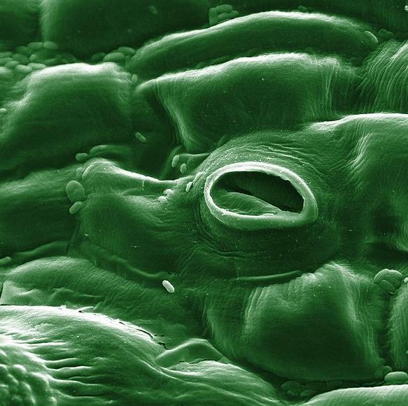
Osmotic pressures at the root zone act to move water into the roots. Once inside the root, water is transported through the plant stem to the intercellular spaces located within the leaves. Air enters the leaves through small surface openings called stoma, plural stomata (Fig. 2-25). Chloroplasts within the leaves use carbon dioxide from the air and a small portion of the available water to manufacture the carbohydrates necessary for plant growth. As air enters the leaf, water escapes through the open stomata and reaches the leaf surface, where it becomes available for evaporation.
The
ratio of water transpired and eventually vaporated to that actually used in plant growth is very large,
up to 800:1 or more [53].
Fig. 2-25 Stoma in a tomato leaf seen through |
Transpiration is a part of plant life and, therefore, it is a continuous process, occurring with or without the presence of precipitation. During a storm, however, interception amounts may use some of the energy available for evaporation, thereby reducing the amount of transpiration. The extent of this effect varies with vegetation type.
Transpiration is also limited by the rate at which moisture becomes available to the plants. Some authorities believe that transpiration is independent of the available soil moisture as long as the latter is above the permanent wilting point, i.e., the soil moisture at which permanent wilting would occur. Others assume that transpiration is roughly proportional to the prevailing soil moisture.
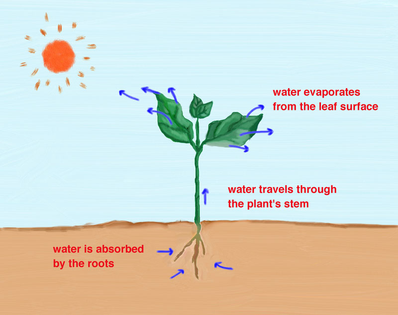
Transpiration rates and amounts vary
widely, depending on vegetation type, depth of root zone, and extent and density of vegetative cover (Fig. 2-26).
Measurements of transpiration are difficult and are usually possible only under highly controlled
circumstances. Since transpiration results in evaporation, transpiration amounts are a function of the
same meteorological and climatic factors that control evaporation rates. In practice, transpiration is
combined with evaporation and expressed as evapotranspiration, which includes all the water converted
into vapor and returned to the atmosphere.
Fig. 2-26 Transpiration. |
In evapotranspiration studies, the concept of potential evapotranspiration (PET) attributed to Thornthwaite [78] is widely used. Potential evapotranspiration is the amount of evapotranspiration that would take place under the assumption of an ample supply of moisture at all times. Therefore, PET is an indication of optimum crop water requirements. In contrast to potential evapotranspiration, actual evapotranspiration is the amount that would take place when water is limiting.
Doorenbos and Pruitt [16] introduced the concept of reference crop evapotranspiration ETo, which is similar to that of potential evapotranspiration. Reference crop evapotranspiration is the rate of evapotranspiration from an extended surface of 8- to 15-cm tall green grass cover of uniform height, actively growing, completely shading the ground, and not short of water. Therefore, the reference crop evapotranspiration can be taken as the potential evapotranspiration of the reference crop (short green grass).
Potential evapotranspiration is equivalent to the evaporation that would occur on a free water surface of extended proportions but of negligible heat storage capacity [50]. Therefore, methods used to calculate potential evapotranspiration resemble the methods used to calculate evaporation. Like evaporation, there are many methods of calculating potential evapotranspiration, each having its own range of applicability. Data requirements vary widely, reflecting the assumptions used in their development.
Most potential evapotranspiration formulas are empirical, dependent upon the known correlation between potential evapotranspiration and one or more meteorological or climatic variables such as radiation, temperature, wind velocity, and vapor pressure difference. Other formulas relate evapotranspiration to direct measurements of water losses using evaporation pans. Models of evapotranspiration and potential evapotranspiration can be grouped into:
- Temperature models,
- Radiation models,
- Combination models, and
- Pan-evaporation models.
It is noted that, when applied to a given set of conditions, the various potential evapotranspiration formulas usually give different estimates. These, however, do not vary widely, with the ratio of maximum and minimum estimates fluctuating throughout the year and rarely exceeding 2:1. As with any such calculation, regional or local experience is required when choosing an appropriate method to calculate potential evapotranspiration.
Temperature Models to Estimate Evapotranspiration. The Blaney-Criddle formula [5, 6] is typical of the temperature models for the estimation of evapotranspiration. The formula has been widely used to estimate crop water requirements. Its original version, applicable on a monthly basis, has the following form:
|
F = P T | (2-39) |
in which F = evapotranspiration for a given month, in inches; P = a day-length variable, defined as the ratio of the total daytime hours for a given month to the total daytime hours in the year, a function of latitude; and T = mean monthly temperature, in degrees Fahrenheit.
In SI units, applicable on a daily basis, the Blaney-Criddle formula is the following:
|
f = p ( 0.46 t + 8.13 ) | (2-40) |
in which f = daily consumptive use factor, in millimeters; p = the ratio of mean daily daytime hours for a given month to the total daytime hours in the year, as a percent, a function of latitude (Table A-3, Appendix A); and t = mean daily temperature for a given month in degrees Celsius.
For a given crop, the consumptive
water requirement is the amount of water required to meet its evapotranspiration needs without
being limited by lack of water. The consumptive water requirement is equal to the product of
consumptive use factor f times an empirical consumptive use crop coefficient
Consumptive
water requirements vary widely between climates having similar air temperatures and day lengths.
Therefore, the effect of climate on crop water requirements is not fully described by the
consumptive use factor f. The effect of climate can be incorporated into the crop coefficient
Doorenbos and Pruitt [16] have proposed a correction to the Blaney-Criddle formula to account for the following local climatic conditions:
- The effect of actual insolation time (the ratio n/N of actual to maximum possible bright sunshine hours),
- Minimum relative humidity φmin in percent (or RH%), and
- Daytime wind speed Ud (measured at a 2-m depth), in m/s.
|
ETo = a + b f | (2-41) |
in which ETo = reference crop evapotranspiration, and a and b are
intercept and slope, respectively, as shown in Fig. 2-27, for three chosen levels of actual
insolation time (low, medium, and high), minimum relative humidity (low, medium, and high),
and daytime wind speed (light, moderate, and strong).
Fig. 2-27 Doorenbos and Pruitt's modification of the Blaney-Criddle formula. |
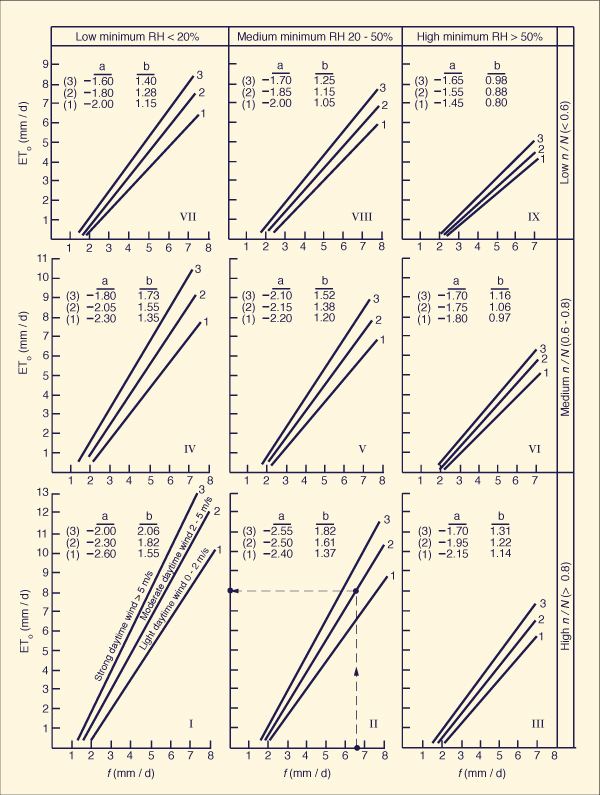
Based on Fig. 2-27, Frevert et al. [20] have developed regression equations for a and b:
|
The consumptive water requirement for a given crop, ETc , can be calculated as follows:
|
ETc = kc ETo | (2-42) |
Approximate range of seasonal crop coefficients are shown in Table 2-7.
|
| |||||||||||||||||||||||||||||||||||||||||||||||||||||||||||||||||||
Example 2-6.
|
The Thornthwaite method is another widely used temperature model to estimate potential evapotranspiration [78]. The method is based on an annual temperature efficiency index J, defined as the sum of twelve (12) monthly values of heat index I. Each index I is a function of the mean monthly temperature T, in degrees Celsius, as follows:
|
T I = ( _____ ) 1.514 5 | (2-43) |
Evapotranspiration is calculated by the following formula:
|
10 T PET (0) = 1.6 ( ______ ) c J | (2-44) |
in which PET (0) = potential evapotranspiration at 0o latitude, in centimeters per month; and c is an exponent to be evaluated as follows:
|
c = 0.000000675 J 3 - 0.0000771 J 2 + 0.01792 J + 0.49239
| (2-45) |
At latitudes other than 0o, potential evapotranspiration is corrected to:
|
PET = K PET (0) | (2-46) |
in which K is a constant for each month of the year, varying as a function of latitude (see Table A-4, Appendix A).
Example 2-7.
|
Radiation Models. Priestley and Taylor [67] proposed that potential evapotranspiration be taken as the radiation part of the Penman equation (Eq. 2-35 with Ea = 0) affected with an empirical constant. Priestley and Taylor's formula is the following:
|
1.26 Δ [ Qn / (ρ H ) ] PET = ________________________ Δ + γ | (2-47a) |
in which PET = potential evapotranspiration, in centimeters per day; Qn = net radiation, in calories per square centimeter per day; Δ is the gradient defined by Eqs. 2-33 and 2-36; and γ is the psychrometric parameter (Table 2-6). Equation 2-47a can also be expressed as follows:
|
1.26 α [ Qn / (ρ H ) ] PET = ________________________ α + 1 | (2-47b) |
in which the constant α can be obtained from Table 2-6.
Recent evaluation of the Priestley-Taylor formula has confirmed its applicability to humid climates. For better estimates in arid climates, the value of the empirical constant should be taken as 1.74 instead of 1.26 [75].
Example 2-8.
|
Pan-evaporation Models.
Evaporation pans provide a measurement of the integrated effect of radiation,
wind, temperature, and humidity on evaporation from an open surface. Plants and vegetation respond to the
same climatic conditions, but several factors produce significant differences in the loss of water. The albedo from
water surfaces is in the range
The basic pan-evaporation formula is the following:
|
PET = Kp Ep | (2-48) |
in which PET = potential evapotranspiration; Kp = pan coefficient; and Ep = pan evaporation.
The most common evaporation pans are the NWS Class A pan and the Colorado sunken pan. The NWS Class A pan
is circular, 122 cm in diameter and 25.4 cm deep, made of galvanized iron (22 gage) or Monel® metal (0.8 mm).
The pan is mounted on a wooden open-frame platform with its bottom 15 cm above ground level. The soil is built
up to within 5 cm of the bottom of the pan, and the pan must be leveled. It is filled with water 5 cm below the
rim, and water level is maintained within 7.5 cm below the rim (Fig. 2-28).
Fig. 2-28 Class A evaporation pan (benmeadows.com). |
The Colorado sunken pan is sometimes preferred in crop water-requirement studies because these pans
tend to yield a better estimate of reference crop
evapotranspiration than the NWS Class A pan. The pan's cross section is a square of side 920 mm and depth 460 mm.
It is made of galvanized iron and set in the ground with the rim 50 mm above ground level (Fig. 2-29). The water inside the
pan is maintained at or slightly below ground level.
Fig. 2-29 Sketch of Colorado sunken pan. |
The pan evaporation approach has been widely used in the determination of potential evapotranspiration. Stanhill [76], for example, concluded that the Class A evaporation pan was the most promising method for estimating potential evapotranspiration. Doorenbos and Pruitt [16] have given guidelines for choosing an appropriate value of pan coefficient for several climatic and site conditions (see Table 2-8).
| |||||||||||||||||||||||||||||||||||||||||||||||||||||||||||||||||||||||||||||||||||||||||||||||||||||||||||||||||||||||||||||||||||||||||||||||||||||||||||||||||||||||||||||||||
2.3 CATCHMENT PROPERTIES
|
|
Surface runoff in catchments occurs as a progression of the following forms, from small to large:
- Overland flow,
- Rill flow,
- Gully flow,
- Streamflow, and
- River flow.
Overland flow is runoff that occurs during or immediately after a storm, in the form of sheet flow over the land surface [Fig. 2-30 (a)]. Rill flow is runoff that occurs in the form of small rivulets, primarily by concentration of overland flow. Gully flow is runoff that has concentrated into depths large enough so that it has the erosive power to carve its own deep and narrow channel (b). Streamflow is concentrated runoff originating in overland flow, rill flow, or gully flow and is characterized by well defined channels or streams of sizable depth (c). Streams carry their flow into larger streams, which flow into rivers to constitute river flow (d).
|
| ||||
|
|
A catchment can range from as little as 1 ha (or acre) to millions of square kilometers (or square miles). [The Amazon basin is 6.915 million km2]. Small catchments (small watersheds) are those where runoff is primarily controlled by overland flow processes. Large catchments (river basins) are those where runoff is controlled by storage processes in the river channels. Between small and large catchments, there is a wide range of catchment sizes with runoff characteristics falling somewhere between those of small and large catchments. In United States practice, midsize catchments are referred to as either watersheds or basins, depending on their drainage area.
Regardless of their size, catchments can drain either inwards, into lakes (or seasonally dry lakes in arid regions), or outwards, and head toward the ocean. Catchments draining inwards have endorheic (or inland continental) drainages (Fig. 2-31). Catchments draining outwards have exorheic (or peripheral continental) drainages. Exorheic drainages have a catchment outlet or mouth at the point of delivery to the next largest stream, and ultimately, to the ocean.
Fig. 2-31 The Great Basin, the largest endorheic basin |
The hydrologic characteristics of a catchment are described in terms of the following properties:
Catchment Area
Area, or drainage area, is perhaps the most important catchment property. It determines the potential runoff volume, provided the storm covers the whole area. The catchment divide is the loci of points delimiting two adjacent catchments, i.e., the collection of high points (peaks and saddles) separating catchments draining into different outlets. Due to the effect of subsurface flow (groundwater flow), the hydrologic catchment divide may not strictly coincide with the topographic catchment divide (Fig. 2-32). The hydrologic divide, however, is less tractable than the topographic divide; therefore, the latter is preferred for practical use.
Fig. 2-32 A river coming out of the ground (Huanuco, Peru). |
The topographic divide is delineated on a quadrangle sheet or other suitable topographic map. The direction of surface runoff is perpendicular to the contour lines. All peaks and saddles are identified at the outset (Fig. 2-33). Runoff from a peak is in all directions; runoff from a saddle is in the two opposing directions perpendicular to the saddle axis. The catchment divide is delineated by joining peaks and saddles with a line which remains perpendicular to the topographic contour. The area enclosed within the topographic divide is measured to determine the catchment area.
Fig. 2-33 Delineation of watershed boundary in Campo Creek, Southeast San Diego County, |
In general, the larger the catchment area, the greater the amount of surface runoff and, consequently, the greater the surface flows. Several formulas have been proposed to relate peak flow to catchment area (Chapter 7). A basic formula is:
|
Qp = c A n | (2-49) |
in which Qp = peak flow, A = catchment area, and c and n are parameters to be determined by regression analysis. Other peak flow methods base their calculations on peak flow per unit area, for instance, the TR-55 method (Chapter 5).
Catchment Shape
Catchment shape is the outline described by the horizontal projection of a catchment. Horton [28] described the outline of a normal catchment as a pear-shaped ovoid. Large catchments, however, vary widely in shape. A quantitative description is provided by the following formula [26]:
|
A Kf = _______ L 2 | (2-50) |
in which Kf = form ratio, A = catchment area, and L = catchment length, measured along the longest watercourse. Area and length are given in consistent units such as square kilometers and kilometers, respectively.
An alternate description is based on catchment perimeter rather than area. For this purpose, an equivalent circle is defined as a circle of area equal to that of the catchment. The compactness ratio is the ratio of the catchment perimeter to that of the equivalent circle. This leads to:
|
0.282 P Kc = ____________ A 1/2 | (2-51) |
in which Kc = compactness ratio, P = catchment perimeter, and A = catchment area, with P and A given in any consistent set of units.
Hydrologic response refers to the relative concentration and timing of runoff (Fig. 2-34). The role of catchment shape in hydrologic response has not been clearly established. Other things being equal, a high form ratio (Eq. 2-50) or a compactness ratio close to 1 (Eq. 2-51) describes a catchment having a fast and peaked catchment response. Conversely a low form ratio or a compactness ratio much larger than 1 describes a catchment with a delayed runoff response. However, many other factors, including catchment relief, vegetative cover, and drainage density are usually more important than catchment shape, with their combined effect not readily discernible.
Fig. 2-34 Hydrologic response of La Leche river basin, Lambayeque, Peru. |
Catchment Relief
Relief is the elevation difference between two reference points. Maximum catchment relief is the elevation difference between the highest point in the catchment divide (Fig. 2-35) and the catchment outlet. The principal watercourse (or main stream) is the central and largest watercourse of the catchment and the one conveying the runoff to the outlet. Relief ratio is the ratio of maximum catchment relief to the catchment's longest horizontal straight distance measured in a direction parallel to that of the principal watercourse. The relief ratio is a measure of the intensity of the erosional processes active in the catchment.
Fig. 2-35 Highest point in the Missouri river basin,
along the border |
The overall relief of a catchment is described by hypsometric analysis [52]. This refers to a dimensionless curve
showing the variation with elevation of the catchment subarea above that elevation (Fig. 2-36). To develop this curve, the
elevation of the highest or maximum point in the catchment divide, corresponding to 0 percent area, is identified.
Also, the elevation of the lowest or minimum point of the catchment, corresponding to 100 percent area, is
identified. Subsequently, several elevations located between maximum and minimum are selected, and the subareas
above each one of these elevations determined by measuring along the respective topographic contour lines. The
elevations are converted to height above minimum elevation and expressed in percentage of the
maximum height. Likewise, the subareas above each one of the elevations are expressed as percentages of total
catchment area. The hypsometric curve shows percent area in the abscissas and percent height in the
ordinates (Fig. 2-36). The median elevation of the catchment is obtained from the percent height corresponding to 50 percent area.
Fig. 2-36 A hypsometric curve. |
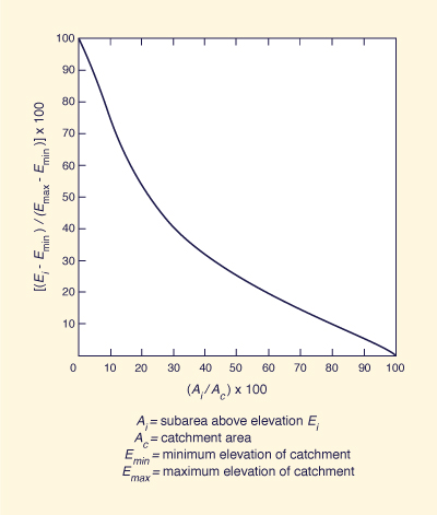
The hypsometric curve is used when a hydrologic variable such as precipitation, vegetative cover, or snowfall shows a marked tendency to vary with altitude. In such cases, the hypsometric curve provides the quantitative means to evaluate the effect of altitude.
Other measures of catchment relief are based on stream and channel characteristics. The longitudinal profile of a channel is a plot of elevation versus horizontal distance (Fig. 2-37). At a given point in the profile, the elevation is usually a mean value of the channel bed. Between any two points, the channel gradient (or channel slope) is the ratio of elevation difference to horizontal distance separating them.
Fig. 2-37 Typical shape of the longitudinal profile of streams and rivers. |
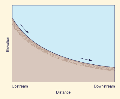
In the absence of geologic controls, longitudinal profiles of streams and rivers are usually concave upward, i.e. , they show a persistent decrease in channel gradient in the downstream direction as the flow moves from mountain streams to river valleys and into the ocean (Fig. 2-37). The reason for this downstream decrease in channel gradient requires careful analysis. It is known that channel gradients are directly related to bottom friction and inversely related to flow depth. Typically, small mountain streams have high values of bottom friction (due to the presence of cobbles and boulders in the stream bed) and small depths [[Fig. 2-38 (a)]. Conversely, large rivers have comparatively lower values of bottom friction and larger depths [Fig. 2-38 (b)]. This interaction of channel gradient and bottom friction helps explain the typical decrease in channel gradient in the downstream direction.
|
|
|
Convex channel bed profiles (Fig. 2-39) are caused by tectonism, uplift, geologic controls, or rock outcrops predominating over an otherwise alluvial channel morphology in equilibrium. These convex stream profiles usually lead to sediment deposition upstream of the outcrop, and to channel erosion immediately downstream.
Fig. 2-39 Bed profile of El Barbon-Guadalupe Creek, Baja California, Mexico. |
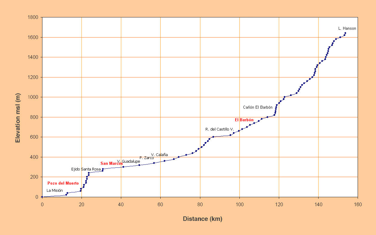
Channels gradients are usually expressed in dimensionless units. For convenience, they can be also expressed in m km-1, cm km-1, or ft mi-1. In nature, channel gradients vary widely, from higher than 0.1 in very steep mountain streams [see, for instance, Fig. 2-38 (a)], to less than 0.000006 in large tidal rivers [19].
In certain unusual geomorphological settings, inland rivers
may feature very small channel gradients; for instance, the Upper
Paraguay river near Porto Murtinho,
Brazil, which
has an average channel slope of
2 cm km-1 (S = 0.00002) (Fig. 2-40).
Fig. 2-40 Upper Paraguay river near Porto Murtinho, Brazil. |
The channel gradient of a principal watercourse is a convenient indicator of catchment relief. A longitudinal profile is defined by its maximum (upstream) and minimum (downstream) elevations, and by the horizontal distance between them (Fig. 2-41). The channel gradient obtained directly from the upstream and downstream elevations is referred to as the S1 slope.
A somewhat more representative measure of channel gradient is the S2 slope, defined as the constant slope that
makes the shaded area above it equal to the shaded area below it (Fig. 2-41). An expedient way to calculate the
S2 slope is to equate the total area below it to the total area below the longitudinal profile.
Fig. 2-41 Sketch of S1 and S2 channel gradients. |
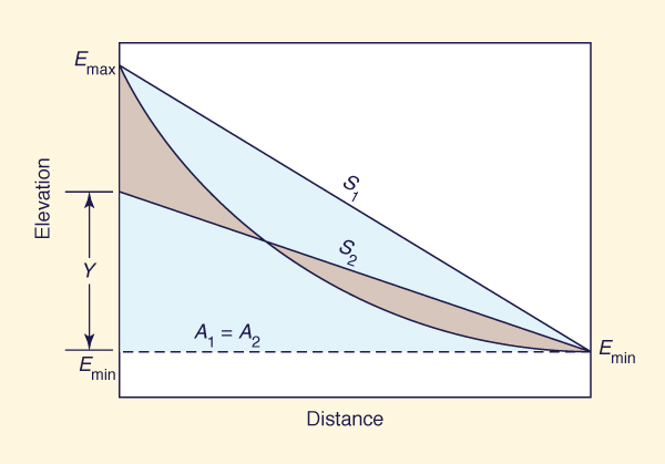
A measure of channel gradient which takes into account the basin response time is the equivalent slope, or S3. To calculate this slope the channel is divided into n subreaches, and a slope is calculated for each subreach. Based on Manning's equation (Section 2.4), the time of flow travel through each subreach is assumed to be inversely proportional to the square root of its slope. Likewise, the time of travel through the whole channel is assumed to be inversely proportional to the square root of the equivalent slope. This leads to the following equation:
|
n Σ Li i = 1 S3 = [ _______________ ] 2 n Σ ( Li / Si 1/2 ) i = 1 | (2-52) |
in which S3 = equivalent slope, Li = each i of n subreach lengths, and Si = each i of n subreach slopes.
Grid methods are often used to obtain measures of land surface slope for runoff evaluations in small and midsize catchments. For instance, the USDA Natural Resources Conservation Service (NRCS) determines average surface slope by overlaying a square grid pattern over the topographic map of the watershed [79]. The maximum surface slope at each grid intersection is evaluated, and the average of all values calculated. This average is taken as the representative value of land surface slope (Fig. 2-42).
Fig. 2-42 Grid overlay to determine land surface slope. |
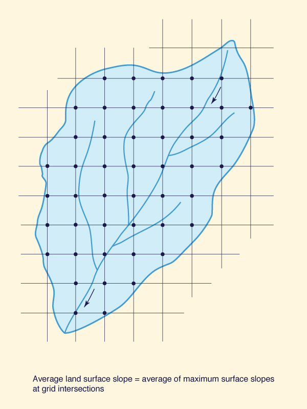
Example 2-9.
|
Fig. 2-43 S1, S2, and S3 channel gradients. |
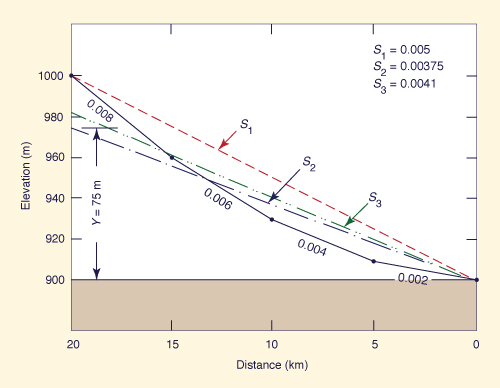
Linear measures are used to describe the one-dimensional features of a catchment. For instance, for small catchments, the overland flow length Lo is the distance of surface runoff that is not confined to any clearly defined channel.
The catchment length (or hydraulic length) L is the length measured along the principal watercourse (Fig. 2-44). The principal watercourse (or main stream) is the central and largest watercourse of the catchment and the one conveying the flow to the outlet.
Fig. 2-44 Linear measures of a catchment. |
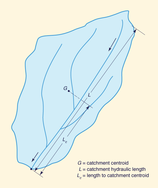
The length to catchment centroid Lc is the length measured along the principal watercourse, from the catchment outlet to a point located closest to the catchment centroid (point G in Fig. 2-44). In practice, the catchment centroid is estimated as the intersecting point of two or more straight lines that bisect the catchment area in approximately equal subareas.
Basin Topology
Basin topology refers to the regional anatomy of the stream network. Distributed rainfall-runoff modeling (Chapter 10) requires the hierarchical description of stream connectivity, i.e., of its topology.
Stream Order. The concept of stream order classifies streams in a network following a hierarchical numbering system. Overland flow can be considered as a hypothetical stream of zero order. A first-order stream is that receiving flow from zero-order streams, i.e., overland flow. Two first-order streams combine to form a second-order stream. In general, two m-order streams combine to form a stream of order m + 1. The catchment's stream order is the order of the most-downstream main stem (Fig. 2-45).
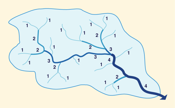
|
Fig. 2-45 Concept of stream order.
A catchment's stream order is directly related to its size. Large catchments may have stream orders of 10 or more. The evaluation of stream order is highly sensitive to map scale. Therefore, considerable care is needed when using stream order analysis in comparative studies of catchment behavior.
Pfasfstetter Coding System. The Pfafstetter coding system is a widely accepted methodology for the description of watershed/basin topology. The system describes the regional anatomy of a stream network using a hierarchical arrangement of decimal digits.
A Level 0 catchment corresponds to a continental-scale size or, alternatively, one that drains into the ocean. Higher levels represent progressively finer subdivisions of the Level 0 catchment. Theoretically, the system is not limited in the number n of levels. In practice, however, n = 6 to 8 levels are usually sufficient. At each level, each watershed is assigned a specific integer m, varying from m = 0 to 9, based on its location and function within the drainage network.
At each level,
watersheds are assigned into three types: (1) basin,
(2) interbasin, and
| ||||||||||||||||||||
For each level, from 1 to n, the assignment of Pfafstetter codes is performed as follows:
From the catchment outlet, trace upstream along the main stem, and identify the four (4) tributaries with the largest drainage areas. The watersheds containing these four tributaries are classified as basins and assigned even digits (m = 2, 4, 6, and 8) from downstream to upstream.
The intervening watersheds, i.e., those contributing lateral inflow to the main stem, are classified as interbasins and assigned odd digits (m = 1, 3, 5, and 7) from downstream to upstream.
The last odd digit m = 9 is reserved for the headwater watershed, i.e., that tributary to interbasin 7.
The largest internal basin, if present, is assigned the number m = 0. Other internal basins, if present, are incorporated into neighboring basins or interbasins.
Figure 2-46 shows a 3-level example of the Pfasfstetter coding system. For each level, say Level 3, the assigned digits (XYm) are appended on to the Level 2 code (XY). For instance, watershed 849 is watershed 8 of Level 1 (coarser), watershed 4 of Level 2 (intermediate), and watershed 9 of Level 3 (finer).
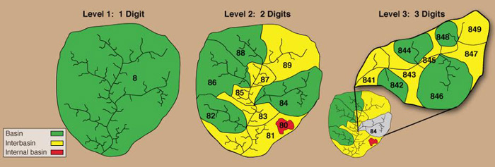
|
Fig. 2-46 The Pfafstetter coding system for watershed identification (Click -here- to display).
Drainage Density
The catchment's drainage density is the ratio of total stream length (the sum of the lengths of all streams) to catchment area. A high drainage density reflects a fast and peaked runoff response, whereas a low drainage density is characteristic of a delayed runoff response.
The mean overland flow length is approximately equal to half the mean distance between stream channels. Therefore, it can be approximated as one-half of the reciprocal of drainage density:
|
1 Lo = _______ 2D | (2-53) |
in which Lo = mean overland flow length, and D = drainage density. This approximation neglects the effect of ground and channel slope, which makes the actual mean overland flow length longer than that estimated by Eq. 2-53. The following equation can be used to estimate overland flow length more precisely:
|
1 Lo = _________________________ 2D [ 1 - (Sc /Sc) ] 1/2 | (2-54) |
in which Sc = mean channel slope, and Ss = mean surface slope.
Drainage Patterns
Drainage patterns in catchments vary widely. The more intricate patterns are an indication of high drainage density. Drainage patterns reflect geologic, soil, and vegetation effects (Fig. 2-47) and are often related to hydrologic properties such as runoff response or annual water yield. Types of drainage patterns that are recognizable on aerial photographs are shown in Fig. 2-48 [30].
Fig. 2-47 Drainage patterns as affected by local geology. |
|
|
| ||||
|
|

Fig. 2-48 Drainage patterns recognizable on aerial photographs.
2.4 RUNOFF
|
|
Surface runoff, or simply runoff, refers to all the waters flowing on the surface of the earth, either by overland sheet flow or by channel flow in rills, gullies, streams, or rivers. Surface runoff is a continuous process by which water is constantly flowing from higher to lower elevations by the action of gravitational forces. Small streams combine to form larger streams which eventually grow into rivers. In time, rivers carry their flow into the ocean, completing the hydrologic cycle.
Runoff is expressed in terms of volume or flow rate. The units of runoff volume are cubic meters, cubic feet, or acre-feet. Flow rate (or discharge) is the volume per unit of time passing through a given area. It is expressed in cubic meters per second or cubic feet per second. Flow rate usually varies in time; therefore, its value at any time is the instantaneous or local flow rate. The local flow rate can be averaged over a period of time to give the average value for that period. The local flow rate can be integrated over a period of time to give the accumulated runoff volume, as follows:
|
∀ = ∫ Q dt
= Σ Q Δt | (2-55) |
in which ∀= runoff volume, Q = flow rate, t = time, and Δt = increment of time.
In engineering hydrology, runoff is commonly expressed in depth units. This is accomplished by dividing the runoff volume by the catchment area to obtain an equivalent runoff depth distributed over the entire catchment.
For certain applications, runoff is alternatively expressed in terms of either: (1) peak flow per unit drainage area, (2) peak flow per unit runoff depth, or (3) peak flow per unit drainage area per unit runoff depth. In the first case, the units are cubic meters per second per square kilometer; in the second case, cubic meters per second per centimeter; in the third case, cubic meters per second per square kilometer per centimeter.
Runoff Components
Runoff may consist of water from three sources:
- Surface flow,
- Interflow, and
- Groundwater flow.
Surface flow is the product of effective rainfall, i.e., total rainfall minus hydrologic abstractions. Surface flow is also called direct runoff. Direct runoff has the capability to produce large flow concentrations in a relatively short period of time. Therefore, direct runoff is largely responsible for flood flows.
Interflow is subsurface flow , i.e., flow that takes place in the vadose zone, i.e., in the unsaturated soil layers located beneath the ground surface (Fig. 2-49). Interflow consists of the lateral movement of water and moisture toward lower elevations, and it includes some of the precipitation abstracted by infiltration. It is characteristically a slow process, but eventually a fraction of the interflow volumes flow into streams and rivers. Typically, the quantities of interflow are relatively small compared to the quantities of surface and groundwater flow.
Fig. 2-49 The vadose zone. |
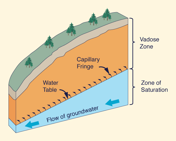
Groundwater flow takes place below the groundwater
table in the form of saturated flow
through alluvial deposits and other water-bearing
geologic formations located beneath the soil mantle
Fig. 2-50 General direction of groundwater flow (U.S. Geological Survey). |
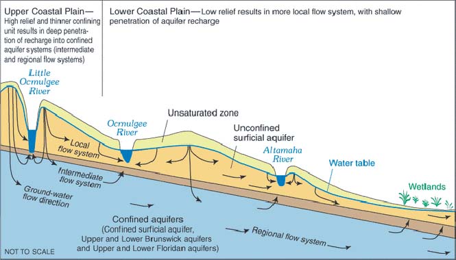
Stream Types and Baseflow
Streams may be grouped into three types:
- Perennial,
- Ephemeral, and
- Intermittent.
Perennial streams are those that always have flow. During dry weather (i.e., absence of rain), the flow of perennial streams is baseflow, consisting mostly of groundwater flow intercepted by the stream. Streams that feed from groundwater reservoirs are called effluent streams. Perennial and effluent streams are typical of subhumid and humid regions [(Fig. 2-51 (a)].
Ephemeral streams are those that have flow only in direct response to precipitation, i.e., during and immediately following a major storm. Ephemeral streams do not intercept groundwater flow and, therefore, have no baseflow. Instead, ephemeral streams usually contribute to groundwater by seepage through their porous channel beds. Streams that feed water into groundwater reservoirs are called influent streams. Channel abstractions from influent streams are referred to as channel transmission losses. Ephemeral and influent streams are typical of arid and semiarid environments [(Fig. 2-51 (b)].
Intermittent streams are those of mixed characteristics, behaving as perennial at certain times of the year and ephemeral at other times. Depending on seasonal conditions, these streams may feed to or from the groundwater [(Fig. 2-51 (c) and (d)].
|
|
| ||||
|
|
Baseflow estimates are important in dry weather hydrology; for instance, in the calculation of the total runoff volume produced by a catchment in a year, referred to as the annual water yield. In flood hydrology, baseflow is used to separate surface runoff into: (a) direct, and (b) indirect runoff. Indirect runoff is surface runoff originating in interflow and groundwater flow. Baseflow is a measure of indirect runoff.
Surface runoff and Baseflow. In practice, surface runoff may or may not include baseflow. The term "surface runoff" is often used at the watershed scale to refer to direct runoff, excluding baseflow. Yet, at the basin scale, estimates of surface water yield typically include both direct runoff and baseflow. The confusion is frequently a source of error in hydrologic analysis. For instance, the NRCS runoff curve number method (Chapter 5) was originally developed to calculate direct surface runoff from small watersheds. Yet, over the years since its original inception, the method has also been used to calculate surface runoff from larger watersheds, which may include baseflow.
Antecedent Moisture
Effective precipitation is the fraction of total precipitation that remains on the catchment surface after all the hydrologic abstractions have taken place. During rainy periods, infiltration plays a major role in abstracting total precipitation. Actual infiltration rates and amounts vary widely, being highly dependent on the initial level of soil moisture. Soil moisture varies with the history of antecedent rainfall, increasing with antecedent rainfall and decreasing with a lack of it. For a given storm, the history of antecedent rainfall, which may have caused the soil moisture to depart from an average state, is termed the "antecedent moisture" or "antecedent rainfall" condition. A catchment with low initial soil moisture (e.g., a catchment drier than normal) is not conducive to high surface flow and direct runoff. Conversely, a catchment with high initial soil moisture (e.g., a catchment wetter than normal) is conducive to large quantities of surface flow and direct runoff (Fig. 2-52).
Fig. 2-52 A catchment with high antecedent moisture: Campo Creek, California, |
The recognition that direct runoff is a function of antecedent moisture has led to the concept of antecedent precipitation index (API). The average moisture level in a catchment varies daily, being replenished by precipitation and depleted by evaporation and evapotranspiration. The assumption of a logarithmic depletion rate leads to a catchment's API for a day with no rain:
|
Ii = K I i-1 | (2-56) |
in which Ii = index for day i, Ii-1 index for day i -1,
and K = a recession factor taken normally in the range
The API is directly related to runoff depth. The greater the value of the index, the greater the amount of runoff. In practice, regression and other statistical tools are used to relate runoff to API. These relations are invariably empirical and therefore strictly applicable only to the situation for which they were derived.
Other measures of catchment moisture have been developed over the years. For instance, the Natural Resources Conservation Service (NSCS) uses the concept of antecedent moisture condition (AMC) (Chapter 5), grouping catchment moisture into three levels: AMC I, a dry condition; AMC II, an average condition; and AMC III, a wet condition. Moisture conditions ranging from AMC II to AMC III are normally used in hydrologic design.
Another example of the use of the concept of antecedent moisture is that of the SSARR model (Chapter 13). The SSARR model computes runoff volume based on a relationship linking runoff percent to a soil-moisture index (SMI), with precipitation intensity as a third variable. Runoff percent is the ratio of runoff to rainfall, multiplied by 100. Such runoff-moisture-rainfall relation is empirical and, therefore, is limited to the basin for which it was derived.
Rainfall can be measured in a relatively simple way. However, runoff measurements usually require an elaborate streamgaging procedure (Chapter 3). This difference has led to rainfall data being more widely available than runoff data. The typical catchment has many more raingages than streamgaging stations, with the rainfall records likely to be longer than the streamflow records.
The fact that rainfall data is more readily available than runoff data has led to the calculation of runoff by relying on rainfall data. Although this is an indirect procedure, it has proven its practicality in a variety of applications.
A basic linear model of rainfall-runoff is the following:
|
Q = b ( P - Pa ) | (2-57) |
in which Q = runoff depth, P = rainfall depth, Pa = rainfall depth below which runoff is zero, and b = slope of the line (Fig. 2-53). Rainfall depths smaller than Pa are completely abstracted by the catchment, with runoff starting as soon as P exceeds Pa. To use Eq. 2-57 it is necessary to collect several sets of rainfall-runoff data and to perform a linear regression to determine the values of b and Pa (Chapter 7). The simplicity of Eq. 2-57 precludes it from taking into account other important runoff-producing mechanisms such as rainfall intensity, infiltration rates, and/or antecedent moisture. In practice, the correlation usually shows a wide range of variation, limiting its predictive ability.
Fig. 2-53 Basic linear model of rainfall-runoff. |

The effect of infiltration rate and antecedent moisture on runoff is widely recognized. Several models have been developed in an attempt to simulate these and other related processes. Typical of such models is the NRCS runoff curve number model, which has had wide acceptance in engineering practice. The NRCS model is based on a nonlinear rainfall-runoff relation that includes a third variable (curve parameter) referred to as runoff curve number, or CN. In a particular application, the CN value is determined by a detailed evaluation of soil type, vegetative and land use patterns, antecedent moisture, and hydrologic condition of the catchment surface. The NRCS runoff curve number method is described in Chapter 5.
Runoff Concentration
An important characteristic of surface runoff is its concentration property. To describe it, assume that a storm falling on a given catchment produces a uniform effective rainfall intensity distributed over the entire catchment area. In such a case, surface runoff eventually concentrates at the catchment outlet, provided the effective rainfall duration is sufficiently long. Runoff concentration implies that the flow rate at the outlet will gradually increase until rainfall from the entire catchment has had time to travel to the outlet and is contributing to the flow at that point. At that time, the maximum, or equilibrium, flow rate is reached, implying that the surface runoff has concentrated at the outlet. The time that it takes a parcel of water to travel from the farthest point in the catchment divide to the catchment outlet is referred to as the time of concentration.
The equilibrium flow rate is equal to the effective rainfall intensity times the catchment area:
|
Qe = Ie A | (2-58) |
in which Qe = equilibrium flow rate; Ie = effective rainfall intensity; and A = catchment area. This equation is dimensionally consistent; however, a conversion factor is needed in the right-hand side to account for the applicable units. For instance, in SI units, with Qe in liters per second, Ie in millimeters per hour, and A in hectares, the conversion factor is 2.78. In U.S. customary units, with Qe in cubic feet per second, Ie in inches per hour, and A in acres, the conversion factor is 1.008, which is often neglected.
The process of runoff concentration can lead to three distinct types of catchment response. The first type occurs when the effective rainfall duration is equal to the time of concentration. In this case, the runoff concentrates at the outlet, reaching its maximum (equilibrium) rate after an elapsed time equal to the time of concentration. Rainfall stops at this time, and subsequent flows at the outlet are no longer concentrated because not all the catchment is contributing. Therefore, the flow gradually starts to recede back to zero. Since it takes the time of concentration for the farthest runoff parcels to travel to the outlet, the recession time is approximately equal to the time of concentration, as sketched in Fig. 2-54. (In practice, due to nonlinearities, actual recession flows are usually asymptotic to zero). This type of response is referred to as concentrated catchment flow.
Fig. 2-54 Concentrated catchment flow. |
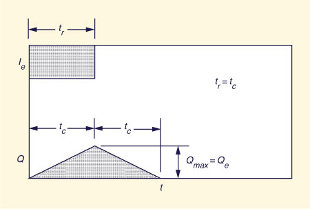
The second type of catchment response occurs when the effective rainfall duration exceeds the time of concentration. In this case, the runoff concentrates at the outlet, reaching its maximum (equilibrium) rate after an elapsed time equal to the time of concentration. Since rainfall continues to occur, the whole catchment continues to contribute to flow at the outlet, and subsequent flows remain concentrated and equal to the equilibrium value. After rainfall stops, the flow gradually recedes back to zero. Since it takes the time of concentration for the farthest runoff parcels to travel to the outlet, the recession time is approximately equal to the time of concentration, as shown in Fig. 2-55. This type of response is referred to as superconcentrated catchment flow.
Fig. 2-55 Superconcentrated catchment flow. |
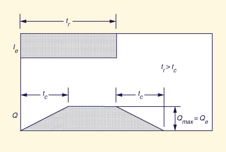
The third type of response occurs when the effective rainfall duration is shorter than the time of concentration. In this case the flow at the outlet does not reach the equilibrium value. After rainfall stops, the flow recedes back to zero. The requirements that volume be conserved and recession time be equal to the time of concentration lead to the idealized flat top response shown in Fig. 2-56. This type of response is referred to as subconcentrated catchment flow.
Fig. 2-56 Subconcentrated catchment flow. |
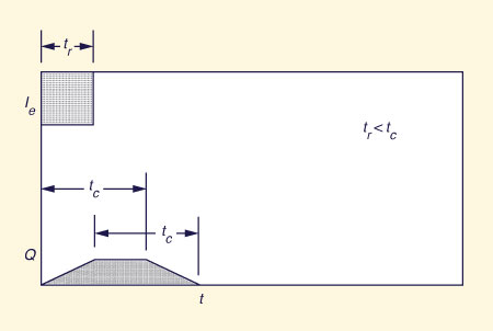
In practice, concentrated and superconcentrated flows are typical of small catchments, i.e., those likely to have short times of concentration. On the other hand, subconcentrated flows are typical of midsize and large catchments, i.e., those with longer times of concentration. Figure 2-57 shows actual dimensionless hydrographs depicting the three types of catchment flows.
Fig. 2-57 Dimensionless hydrographs showing three types of catchment flow. |
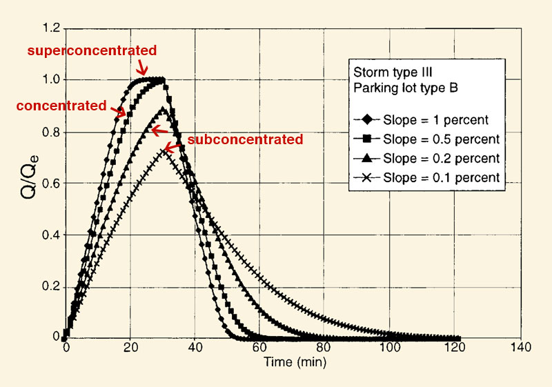
Time of Concentration. Hydrologic procedures for small catchments usually require an estimate of the time of concentration (Chapter 4). However, precise estimations are generally difficult. For one thing, time of concentration is a function of runoff rate; therefore, an estimate can only represent a certain flow level, whether it be low flow, average flow, or high flow.
Several formulas for the calculation of time of concentration are available. Most are empirical in nature and, therefore, of somewhat limited value. Nevertheless, a few are widely used in practice. An alternate approach is to calculate time of concentration by dividing the principal watercourse into several subreaches and assuming an appropriate flow level for each subreach. Subsequently, a steady open-channel flow formula such as the Manning equation is used to calculate the mean velocity and associated travel time through each subreach. The time of concentration for the entire reach is the sum of the times of concentration of the individual subreaches. This procedure, while practical, is based on several assumptions, including a flow-rate level, a prismatic channel, and Manning's n values.
A limitation of the steady flow approach to the calculation of time of concentration is the fact that the flow being considered is generally unsteady. This means that the speed of travel of the wavelike features of the flow (i.e., the kinematic wave speed, Chapters 4 and 9) is greater than the mean velocity calculated using steady flow principles (the Manning equation). For instance, for turbulent flow in hydraulically wide channels, kinematic wave theory justifies a wave speed as much as 5/3 times the mean flow velocity, with a consequent reduction in travel time and associated time of concentration. Yet, in many cases, the ratio between kinematic wave speed and mean flow velocity is likely to be less than 5/3:1. In practice, the uncertainties involved in the computation of time of concentration have contributed to a blurring of the distinction between the two speeds.
Formulas for Time of Concentration. Notwithstanding the inherent complexities, calculations of time of concentration continue to be part of the routine practice of engineering hydrology. The time of concentration is a key element in the rational method (Chapter 4) and other methods used to calculate the runoff response of small catchments. Most formulas relate time of concentration to suitable length, slope, roughness, and rainfall parameters [62]. A well-known formula which relates time of concentration to length and slope parameters is the Kirpich formula, applicable to small agricultural watersheds with drainage areas less than 8 acres (200 ha) [46]. In SI units, the Kirpich formula is:
|
L 0.77 tc = 0.06628 ___________ S 0.385 | (2-59) |
in which tc = time of concentration, in hours; L = length of the principal watercourse, from divide to outlet, in kilometers; and S = slope between maximum and minimum elevation (S1 slope), in meters per meter. In U.S. customary units, with tc in minutes, L in feet and S in feet per foot, the coefficient of Eq. 2-83 is 0.0078.
The Kerby-Hathaway formula relates time of concentration to length, slope, and roughness parameters as follows [22]:
|
( L n ) 0.467 tc = 0.606 _______________ S 0.234 | (2-60) |
in which n is a roughness parameter and all other terms are the same as in Eq. 2-59, expressed in SI units. Applicable values of n are given in Table 2-10.
| |||||||||||||||||
The Papadakis-Kazan formula [62] relates time of concentration to length, slope, roughness, and rainfall parameters:
|
L 0.50 n 0.52 tc = 0.66 _________________ S 0.31 i 0.38 | (2-61) |
in which tc is in minutes; L is in feet; n is a roughness parameter; and i is the effective rainfall in inches per hour.
A physically based approach to the calculation of time of concentration is possible by means of overland flow techniques (Chapter 4). As a first approximation, time of concentration can be taken as the time-to-equilibrium of kinematic overland flow (Eq. 4-50). Therefore:
|
(L n) 1/m tc = ______________________ S 1/(2 m) i (m - 1)/m | (2-62) |
in which tc is given in seconds; L is in meters; n is a roughness parameter, i is in m/s, and m = exponent of the unit-width discharge-flow depth rating (q = b h m ).
For m = 5/3, applicable to turbulent Manning friction (in hydraulically wide channels), the kinematic wave time of concentration is:
|
(L n) 0.6 tc = ______________ S 0.3 i 0.4 | (2-63) |
in which tc is in seconds; L is in meters; n is a roughness parameter; and i is the effective rainfall in meters per second. The close resemblance of the exponents of Eqs. 2-61 and 2-63 is remarkable.
Use the Kirpich, Hathaway, Papadakis-Kazan, and kinematic wave formulas to estimate
time of concentration for a catchment with the following characteristics: L = 750 m, S = 0.01,
n = 0.1, and i = 20 mm hr -1.
After conversion to the proper units,
the application of
ONLINE CALCULATION. Using ONLINE TIME OF CONCENTRATION, the answer
is:
Kirpich ⇒
Example 2-10.
![]()
Runoff Diffusion and Streamflow Hydrographs
In nature, catchment response shows a more complex behavior than that which may be attributed solely to runoff concentration. Theory and experimental evidence have shown that runoff rates are governed by natural processes of convection and diffusion. Convection refers to runoff concentration; diffusion is the mechanism acting to spread the flow rates in time and space.
The net effect of runoff diffusion is to reduce the flow rates to levels below those that could be attained by convection only. In practice, diffusion acts to smooth out catchment response. The resulting response function is usually continuous, and it is referred to as the streamflow hydrograph, runoff hydrograph, or simply the hydrograph. Typical single-storm hydrographs have a shape similar to that shown in Fig. 2-58. They are usually produced by storms with effective rainfall duration less than the time of concentration. Therefore, they resemble subconcentrated catchment flow, albeit with the addition of a small but perceptible amount of diffusion.
Fig. 2-58 Typical single-storm hydrograph. |
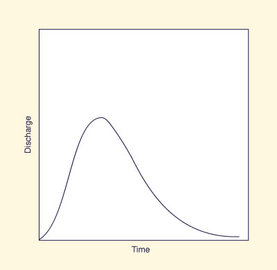
The various elements in a typical single-storm hydrograph are shown in Fig. 2- 59. The zero time (or starting time) depicts the beginning of the hydrograph. The hydrograph peak describes the maximum flow rate. The time-to-peak is measured from zero time to the time at which the peak flow is attained. The rising limb is the part of the hydrograph between zero time and time-to-peak. The recession (or receding limb) is the part of the hydrograph between time-to-peak and time base. The time base is measured from zero time to a time defining the end of the recession. The recession is logarithmic in nature, approaching zero flow in an asymptotic way. For practical applications, the end of the recession is usually defined in an arbitrary manner. The point of inflection of the receding limb is the point corresponding to zero curvature. The hydrograph volume is obtained by integrating the flow rates from zero time to time base.
Fig. 2-59 Elements of single-storm hydrograph. |
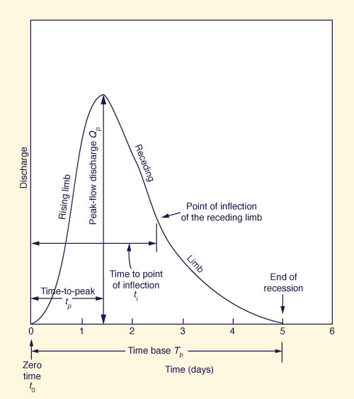
The shape of the hydrograph, showing a positive skew, with recession time greater than rising time, is caused by the essentially different responses of surface flow, interflow, and groundwater flow. Indeed, the runoff hydrograph can be thought of as consisting of the sum of up to three hydrographs, as shown in Fig. 2-60 (a). The fast and peaked hydrograph is produced by surface flow while the other two are the result of interflow and groundwater flow. The superposition of these hydrographs results in a runoff hydrograph exhibiting a long tail (positive skew), as depicted in Fig. 2-60 (b).
Fig. 2-60 Components of runoff hydrograph. |
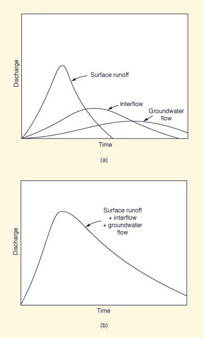
The feature of positive skew allows the definition of a few additional geometric hydrograph properties. The time-to-centroid tg is measured from zero time to the time separating the hydrograph into two equal volumes (Fig. 2-61). The volume-to-peak Vp is obtained by integrating the flow rates from zero time to time-to-peak. In synthetic unit hydrograph analysis, the ratio of volume-to-peak to hydrograph volume is used as a measure of hydrograph shape (Chapter 5).
Fig. 2-61 Additional single-storm hydrograph properties. |
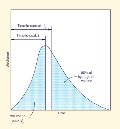
Hydrographs of perennial streams may include substantial amounts of baseflow. The separation of runoff into direct runoff (surface flow) and indirect runoff (baseflow) can be accomplished by resorting to one of several hydrograph separation techniques (Chapter 5). These techniques can also be used in the analysis of multiple-storm hydrographs, which typically exhibit two or more peaks and valleys.
Analytical Hydrographs. Analytical expressions for streamflow hydrographs are sometimes used in hydrologic studies. The simplest formula is based on either a sine or cosine function. These, however, have zero skew (Chapter 6) and therefore do not properly describe the shape of natural hydrographs.
An analytical hydrograph that is often used to simulate natural hydrographs is the gamma function, expressed as follows:
|
t Q = Qb + (Qp - Qb ) [ _____ ] m e (tp - t ) / (tg - tp ) tp | (2-64) |
in which Q = flow rate; Qb = baseflow; Qp = peak flow; t = time; tp = time-to-peak; tg = time-to-centroid; and m = tp /(tg - tp). For values of tg greater than tp, Eq. 2-64 exhibits positive skew.
Example 2-11.
|
| ||||||||||||||||||||||||||||||||||||
Flow in Stream Channels
Streamflow hydrographs flow in stream channels that are carved on the land surface. The following properties are used to describe stream channels:
- Cross-sectional dimensions,
- Cross-sectional shape,
- Longitudinal slope, and
- Boundary friction.
The channel cross section has the following geometric and hydraulic elements: (a) flow area, (b) top width, (c) wetted perimeter, (d) hydraulic radius, (e) hydraulic depth, and (f) aspect ratio. The flow area A is the area of the cross section occupied by the flow. The top width T is the channel width at the elevation of the water surface. The wetted perimeter P is the perimeter of the flow area in direct contact with the land. The hydraulic radius R is the ratio of flow area to wetted perimeter: R = A/P. The hydraulic depth D is the ratio of flow area to top width: D = A/T. The aspect ratio, a measure of cross-sectional shape, is the ratio of top width to hydraulic depth (T/D).
Channel top widths vary widely, ranging from a few meters for small mountain streams to several kilometers for very large rivers. Mean flow depths range from as low as a fraction of a meter for small mountain streams to more than 50 m for very large rivers. [The maximum depth of the Amazon river, the largest in the world, is close to 90 m]. Aspect ratios vary widely in nature; however, most streams and rivers have aspect ratios in excess of 10. Very wide streams (e.g., braided streams) may have aspect ratios exceeding 100.
The longitudinal channel slope is the change in elevation with distance. The mean bed elevation is generally used to calculate channel slope. For short reaches or mild slopes, slope calculations may be hampered by the difficulty of accurately establishing the mean bed elevation. A practical alternative is to use the water surface slope as a measure of channel slope. The water surface slope, however, varies in space and time as a function of the flow nonuniformity and unsteadiness. The steady equilibrium (i.e., uniform) water surface slope is usually taken as a measure of channel slope. Therefore, mean bed slope and steady equilibrium water surface slope are often treated as synonymous. Generally, the longer the channel reach, the more accurate the determination of channel slope.
Boundary friction refers to the type and dimensions of the particles lining the channel cross section below the waterline. In alluvial channels, geomorphic bed features such as ripples and dunes may represent a substantial contribution to the overall friction (Chapter15). Particles lying on the channel bed may range from large boulders for typical mountain streams (Fig. 2-62) to silt particles in the case of large tidal rivers.
Fig. 2-62 Flow in a mountain stream. |
For small streams, particles on the channel banks may be as large as the particles on the bottom. River banks, however, are likely to consist of particles of much varied size than those on the channel bottom. The high aspect ratio of rivers generally results in the banks contributing only a small fraction of the total boundary friction. Therefore, the boundary friction is often taken as synonymous with bed or bottom friction.
Uniform flow formulas. Flow in streams and rivers is evaluated by using empirical formulas such as the Manning or Chezy equations. The Manning formula is:
|
1 V = _____ R 2/3 S 1/2 n | (2-65) |
in which V = mean flow velocity, in meters per second; R = hydraulic radius, in meters; S = channel slope, in meters per meter; and n = Manning friction coefficient. In U.S. customary units, with V in feet per second, R in feet, and S in feet per foot, the right side of Eq. 2-65 is multiplied by the constant 1.486.
In natural channels, n can take values as low as 0.02 and as high as 0.2 in some unusually high roughness cases (e.g., flood plains adjacent to rivers). A good working value for a clean, straight, full-stage stream of fairly uniform cross section is 0.03. Typical n values for natural streams and rivers are in the range 0.03-0.05.
A U.S. Geological Survey study [4] has documented n values for natural streams ranging from as low as n = 0.024 for the Columbia River at Vernita, Washington (a large river with streambanks largely devoid of vegetation) [(Fig. 2-63 (a)], to as high as n = 0.079 for Cache Creek near Lower Lake, California (a small stream with large, angular boulders in the bed, and exposed rocks, boulders, and trees in the banks) [(Fig. 2-63 (b)].
|
|
|
The Chezy equation is
|
V = C R 1/2 S 1/2 | (2-66) |
in which C = Chezy coefficient, in m1/2 s-1; and other terms are the same as for Eq. 2-65. Chezy coefficients equivalent to the preceding conditions range from about 80 m1/2 s-1 for large rivers to about 10 m1/2 s-1 for small streams. Typical C values for natural streams and rivers are in the range 25-50 m1/2 s-1.
Equation 2-66 can be expressed in dimensionless form as follows:
|
C V = _______ g 1/2 R 1/2 S 1/2 g 1/2 | (2-67) |
in which g = gravitational acceleration, and C/g1/2 = dimensionless Chezy coefficient. Dimensionless Chezy coefficients equivalent to the preceding conditions range from 25.5 for large rivers to 3.2 for small streams. Typical values for natural streams and rivers are in the range 8-16.
For certain applications, Eq. 2-67 can be readily transformed into a formula with an enhanced physical meaning. For hydraulically wide channels, i.e., those with aspect ratio greater than 10, the top width and wetted perimeter can be assumed to be approximately the same. This implies that the hydraulic depth (D) can be substituted for the hydraulic radius (R), leading to:
|
S = f F 2 | (2-68) |
in which f = a dimensionless friction factor equal to f =
g/C 2, and F =
Froude number, equal to
Equation 2-68 states that for hydraulically wide channels, the channel slope is proportional to the square of the Froude number, with the friction factor f as the proportionality coefficient. In practice, Eq. 2-68 be used as a convenient predictor of any of these three dimensionless parameters, once the other two are known. Furthermore, it implies that if one of the three parameters is kept constant, a change in one of the other two causes a corresponding change in the third.
Notwithstanding the theoretical appeal of Eqs. 2-66 and 2-68, the Manning equation has had wider acceptance in practice. This is attributed to the fact that in natural channels, the Chezy coefficient is not constant, tending to increase with hydraulic radius. The comparison of Eqs. 2-65 and 2-66 leads to:
|
1 C = _____ R 1/6 n | (2-69) |
Equation 2-69 implies that, unlike Chezy C, Manning n is a constant. Experience has shown, however, that at a given cross-section, n may vary with discharge and stage (Fig. 2-64). Moreover, as stage varies from low to high, alluvial rivers can move their beds and generate/erase ripples and dunes, increasing/decreasing channel friction (Chapter 15).
Fig. 2-64 A large river overflowing onto the adjacent flood plain (Mato Grosso, Brazil). |
River Stages. At any location along a river, the river stage is the elevation of the water surface above a given datum. This datum can be either an arbitrary one or the NAVD (North American Vertical Datum), a standard measure of mean sea level.
River stages are a function of flow rate. Flow rates can be grouped into: (1) low flow, (2) average flow, and (3) high flow. Low flow is typical of the dry season, when streamflow is largely composed of baseflow originating mostly in contributions from groundwater flow. High flow occurs during the wet season, when streamflow is primarily due to contributions from surface runoff. Average flow usually occurs midseason and may have mixed contributions from surface runoff, interflow, and groundwater flow.
Low flows studies are necessary when determining minimum flow rates, below which a certain use would be impaired. Examples of such uses are irrigation requirements, hydropower generation, and minimum instream flows needed for fisheries protection and compliance with water pollution regulations. Excessive use of groundwater may lead to baseflow losses; thus, Increasingly, surface runoff studies are focusing on baseflow and low flows.
Average flows play an important role in the calculation of monthly and annual volumes available for storage and use. Applications are usually found in connection with the sizing of storage reservoirs.
High flow studies are related to the floods and flood hydrology. Typically, during high flows, natural streams and rivers have the tendency to overflow their banks, with stages reaching above bank-full stage. In such cases, the flow area includes a portion of the land located adjacent to the river, on one or both sides. In alluvial valleys, the land that is subject to inundation during periods of high flow is referred to as the flood plain (Fig. 2-65). The evaluation of high flows is necessary for flood forecasting, flood control, and flood mitigation.
Fig. 2-65 Flood plain flooding (Mato Grosso, Brazil). |
Rating Curves. It is known that river stage varies as a function of discharge, but the exact nature of the relationship is not readily apparent. Given a long and essentially prismatic channel reach, a single-valued relationship between stage and discharge at a cross section defines the equilibrium rating curve. For steady uniform flow, the rating curve is unique, i.e., there is a single value of stage for each value of discharge and vice versa (Fig. 2-66). In this case, the equilibrium rating curve can be calculated with either the Manning or Chezy equations. In open-channel hydraulics, this property of uniqueness of the rating qualifies the channel reach as a channel control.
Fig. 2-66 A typical rating curve. |
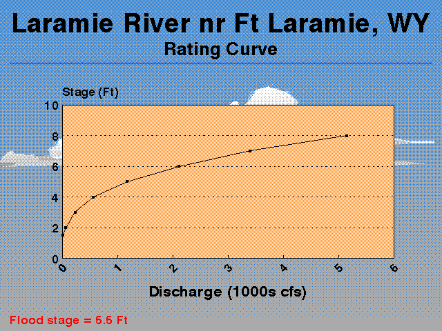
However, other flow conditions, specifically nonuniformity (gradually varied steady flow) and unsteadiness (e.g., gradually varied unsteady flow), can cause deviations from the steady equilibrium rating. These deviations are less tractable. In particular, flood wave theory justifies the presence of a loop in the rating, as shown in Fig. 2-67. Intuitively, the rising limb of the flood-wave hydrograph has a steeper water surface slope than that of equilibrium flow, leading to greater flows and lower stages. Conversely, the receding limb has a milder water surface slope, resulting in smaller flows and higher stages; thus the rationale for the loop's presence. The loop effect, however, is likely to be small and is usually neglected on practical grounds. Where increased accuracy is required, unsteady flow modeling can be used to account for the looped rating (Chapter 9).
Fig. 2-67 A looped rating curve. |
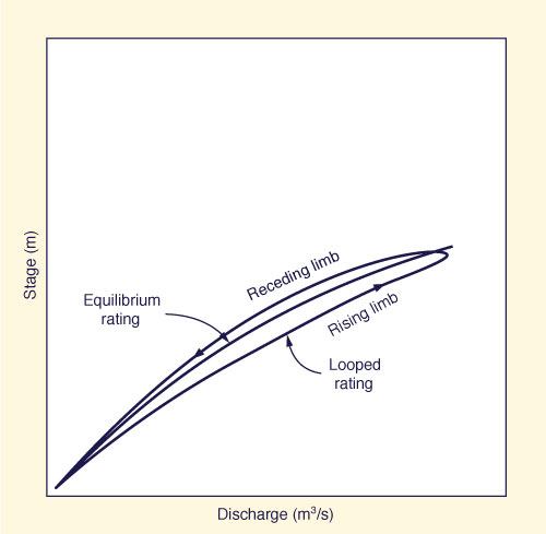
Two other processes related to sedimentation have a bearing in the evaluation of stage-discharge relations: (1) the short-term effects, and (2) long-term effects. The short-term effects are due to the fact that the amount of boundary friction varies with flow rate. Rivers flowing on loose boundaries composed of gravel, sand, and silt constantly try to minimize their changes in stage. This is accomplished through the following mechanism: During low flow, the bed friction consists not only of grain friction but also of form friction, caused by bed features such as ripples and dunes (Chapter 15). During high flows, the swiftness of the current acts to obliterate the bed features, reducing form friction to a minimum, essentially with only grain friction remaining. The reduced friction during high flows gives rivers the capability to carry a greater discharge for a given stage. This explains the demonstrated shift from low-flow rating to high-flow rating in natural river channels (Fig. 2-63).
The long-term sedimentation effect is due to the fact that rivers continuously subject their boundaries to recurring cycles of erosion and deposition, depending on the sediment load they carry (Chapter 15). Some very active rivers may be eroding; others may be aggrading. Moreover, some geomorphologically active rivers may substantially change their cross sections during major floods. Invariably, shifts in rating are the net result of these natural geomorphic processes.
Rating Curve Formulas. In spite of the apparent complexities, rating curves are a useful and practical tool in hydrologic analysis, allowing the direct conversion of stage to discharge and vice versa. Discharge can be obtained from the rating by the simple procedure of measuring the stage. Conversely, if discharge is known, for instance, at a catchment outlet, stage at the outlet can be readily determined from a suitable rating.
There are several ways to determine an equation for the rating. Invariably, they are based on curve-fitting stage-discharge data. A widely used equation is the following [45]:
|
Q = a (h - ho ) b | (2-70) |
in which Q = discharge; h = gage height; ho = reference height; and a and b are constants. Several values of reference height are tried. The proper value of reference height is that which makes the stage-discharge data plot as close as possible to a straight line on logarithmic paper. Subsequently, the values of the constants a and b are determined by regression analysis (Chapter 7).
Streamflow Variability
The study of streamflow variability is the cornerstone of engineering hydrology. Streamflow and river flow vary not only seasonally, but also annually, multiannually, and with climate and geographic location. Global climate change may also affect streamflow variability. Over the long term, the total amount of streamflow is directly related to the amount of environmental moisture, i.e., the moisture present in soil and air. The inland advection of water vapor supplies the moisture which eventually constitutes precipitation. Whether this moisture reaches the catchment outlet remains to be determined by further analysis.
On an average global basis, mean annual runoff, measured at the mouths of peripheral continental basins, amounts to about 39 percent of total precipitation. Most of the remainder, about 59 percent, is accounted for by the long-term abstractive processes of evaporation and evapotranspiration, which include evaporation from water bodies, evaporation from soil and bare ground, and evapotranspiration from vegetation. A small percentage, about 2 percent, percolates deep enough into the ground to bypass the surface waters, eventually discharging into the ocean (Fig. 2-68).
Fig. 2-68 Average global components of the water balance. |
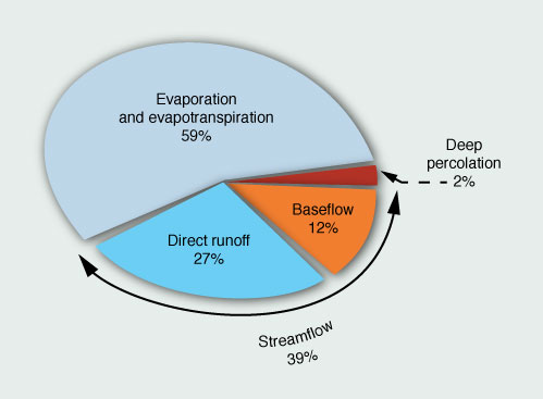
Seasonal Variability. A typical catchment in a subhumid region may show runoff rates and volumes varying throughout the year, with a tendency to low flows during the dry season and high flows during the wet season. However, a catchment in a more extreme climate will show a quite different behavior. In the ephemeral streams typical of arid regions, runoff is nonexistent during periods of no precipitation; for these streams, runoff occurs only in direct response to precipitation. On the other hand, in humid and extremely humid climates, rivers show substantial amounts of runoff throughout the year, with relatively little variability between the seasons.
The reason for the seasonal variability of streamflow lies in the relative contributions of direct (surface flow) and indirect runoff (baseflow). In subhumid regions, indirect runoff is a small, but nevertheless measurable, fraction of total runoff. On the other hand, in arid regions, particularly for ephemeral streams, indirect runoff is either zero or negligible. Furthermore, in humid regions, indirect runoff is substantial throughout the year, often being a sizable fraction of total runoff.
The phenomenon described above can be further explained in the following way: Groundwater reservoirs act to store large amounts of water, which are slowly transported to lower elevations. The bulk of this water (about 98% on a global basis) is eventually released back to the surface waters. With seepage being the dominant process, the flow of groundwater is slow and, therefore, subject to a substantial amount of diffusion. The net effect is that of a permanent contribution from groundwater to surface water in the form of baseflow, or the dry-weather flow of rivers (Fig. 2-69). To evaluate the seasonal variability of streamflow, it is therefore necessary to examine the relationship between surface water and groundwater.
Fig. 2-69 Large spring contributing to baseflow. |
Annual Variability. Year-to-year streamflow variability shows some of the same features as those of seasonal streamflow variability. For instance, large catchments show runoff variability from one year to the next as a function of the state of moisture at the end of the first year and of the precipitation amounts added during the second year. As in the case of seasonal variability, annual streamflow variability is linked to the relative contributions of direct and indirect runoff. During dry years, precipitation goes on to replenish the catchment's soil moisture deficit, with little of it showing as direct runoff. This results in the low levels of runoff that characterize dry years. Conversely, during wet years, the catchment's moisture storage capacity fills up quickly, and any additional precipitation is almost entirely converted into surface runoff. This produces the high streamflow levels that characterize wet years. Annual streamflow variability is, therefore, intrinsically connected to the relative contributions of direct and indirect runoff.
An increasingly popular line of inquiry is to focus on the mechanics of surface flow, interflow, and groundwater flow, while accounting for the spatial and temporal variability of the various physical, chemical, and biological processes involved at the various scales. However, the dearth of reliable data for all phases of the hydrologic cycle makes the evaluation of streamflow using a purely mechanistic approach a rather complex undertaking. Recent progress has been made in the coupling of mathematical models with geographic information systems, digital elevation models, and other related software.
A practical alternative which has enjoyed wide acceptance in applications of flood hydrology is the reliance on statistical tools to compensate for the incomplete knowledge of the physical processes. Over the years, this has given rise to the concept of flow frequency, or commonly, flood frequency, expressed as the average period of time (i.e., the return period) that it will take a certain flood level to recur at a given location. An annual flood series is abstracted from daily discharge measurements at a given gaging station. This is accomplished by either selecting the maximum daily flow for each of n years of record (the annual maxima series), or by selecting the n greatest flow values in the entire n-year record, regardless of when they occurred (the annual exceedance series) (Chapter 6). The statistical analysis of the flood series permits the calculation of the flow rates associated with one or more chosen frequencies.
The procedure is relatively straightforward, but it is limited by the record length. Its predictive capability decreases sharply when used to evaluate floods with return periods substantially in excess of the record length. An advantage of the method is its reproducibility, which means that two persons are likely to arrive at the same result when using the same methodology. This is a significant asset when comparing the relative merits of competing water resources projects. Methods for flood frequency analysis are discussed in Chapter 6.
Recently, a complicating factor has arisen in flood frequency analysis. Global climate change promises to change the long-term depth-duration-frequency precipitation relations and, therefore, the magnitude and frequency of floods. Then, a historical flood record, however long, would have essentially lost its pristine character and could only serve as a rough indication for present and future analyses.
Daily-flow Analysis. The variability of streamflow can also be expressed in terms of the day-to-day fluctuation of flow rates at a given station. Some streams show great variability from day to day, with high peaks and low valleys succeeding one another endlessly. Other streams show very little day-to-day variability, with high flows being not very different from low flows.
The reason for this difference in behavior can be attributed to differences in the nature of catchment response. Small and midsize catchments are likely to have steep gradients and therefore to concentrate flows with negligible runoff diffusion, producing hydrographs that show a large number of high peaks and corresponding low valleys. Conversely, large catchments are likely to have milder gradients and therefore to concentrate flows with substantial runoff diffusion. The diffusion mechanism acts to spread the flows in time and space, resulting in a succession of smooth hydrographs showing low peaks and comparatively high valleys.
Daily flow data may not be sufficient to allow calculation of the runoff volumes produced by small watersheds. In cases where accuracy is required, hourly flows (or perhaps flows measured at 3-h intervals) may be necessary to describe adequately the temporal variability of the flow.
In the past four decades, the development of stochastic models of streamflow variability has resulted in a substantial body of knowledge referred to as stochastic hydrology. For a detailed treatment of this subject, see [8, 70, 89].
Flow-duration Curve. A practical way to evaluate day-to-day streamflow variability is the flow-duration curve. To determine this curve for a particular location, it is necessary to obtain daily flow data for a certain period of time. either 1 y or a number of years. The length of the record indicates the total number of days in the series. The daily flow series is sequenced in decreasing order, from the highest to the lowest flow value. with each flow value being assigned an order number. For instance, the highest flow value would have order number one; the lowest flow value would have the last order number, equal to the total number of days. For each flow value, the percent time is defined as the ratio of its order number to the total number of days, expressed in percentage. The flow-duration curve is obtained by plotting flow versus percent time, with percent time in the abscissas and flow in the ordinates (Fig. 2-70).
Fig. 2-70 A flow-duration curve. |
A flow-duration curve allows the evaluation of the permanence of characteristic low-flow levels. For instance, the flow expected to be exceeded 90 percent of the time can be readily determined from a flow-duration curve. The permanence of low flows is increased with streamflow regulation. The usual aim is to be able to assure the permanence of a certain low-flow level 100 percent of the time. Regulation causes a shift in the flow-duration curve by increasing the permanence of low flows while decreasing that of high flows (Fig. 2-67). Streamflow regulation is accomplished with storage reservoirs.
The flow-duration curve is helpful in the planning and design of water resources projects. In particular, for hydropower studies, the flow-duration curve serves to determine the potential for firm power generation. In the case of a run-of-the-river plant, with no storage facilities, the firm power is usually assumed on the basis of flow available 90 to 97 percent of the time.
Flow-mass Curve. Another way to evaluate day-to-day (and seasonal) streamflow variability is the flow-mass curve. A mass curve of daily values of a variable is a plot of time in the abscissas versus cumulative values of the variable in the ordinates. When using flow values, such a plot is referred to as the flow-mass curve.
For daily flow records in cubic meters per second, the ordinates of the flow mass curve are in cubic meters or cubic hectometers (1 cubic hectometer = 1 million cubic meters). For any given day, the ordinate of the flow-mass curve is the accumulated runoff volume up to that day. According to Chow [10], the flow-mass curve is believed to have been first suggested by Rippl [69]; hence the name Rippl curve. The shape of the flow-mass curve resembles that of the letter S (Fig. 2-71); therefore, it is also referred to as the S-curve.
Applications of flow-mass curves are to reservoir design and operation, including the determination of reservoir capacity and the establishment of operating rules for storage reservoirs. Figure 2-71 shows a typical flow-mass curve. At any given time, the slope of the mass curve is a measure of the instantaneous flow rate. The slope of the line PQ, drawn between the points P and Q, represents the average flow between the two points. The slope of the line AB, drawn between the starting point A and the ending point B, is the average flow for the entire period.
Fig. 2-71 A typical flow-mass curve. |
To use the flow-mass curve for reservoir design, two lines parallel to line AB and tangent to the flow-mass curve are drawn (Fig. 2-71). The first one, A'B', is tangent to the mass curve at the highest tangent point C. The second one, A"B", is tangent to the mass curve at the lowest tangent point D. The vertical difference between these two tangent lines, in cubic meters, is the storage volume required to release a constant flow rate. This constant release rate is equal to the slope of the line AB. A reservoir with a volume equal to AA" at the start would be full at C and empty at D, with no spill (excess volume) or shortage (deficit). A reservoir that is empty at the start has water while the S curve remains above the AB line and is empty (show a deficit) when the S curve moves below that line. A reservoir that is full at the start will spill water (excess volume) as long as the inflow remains greater than the outflow (from A to C).
The draft rate (or demand rate) is the release rate required to fulfill downstream needs, such as irrigation or power generation. A line having a slope equal to the draft rate is the draft line. The draft rate need not be necessarily constant. In practice, reservoir withdrawals are variable, leading to a variable draft rate and variable draft line, which amounts to an outflow mass curve. The superposition of inflow and outflow mass curves enables the detailed analysis of reservoir storage.
The residual mass curve is a plot of the differences between the S curve ordinates and the corresponding ordinates from line AB. The ordinates of the residual mass curve can be either positive or negative. The residual mass curve accentuates the peaks and valleys of the cumulative flow record.
Range is the difference between the maximum and minimum ordinates of the residual mass curve for a given period. Range analysis was pioneered by Hurst [31, 32] who proposed the following formula for the calculation of maximum range:
|
N R = s ( _____ ) 0.73 2 | (2-71) |
in which R = reservoir storage volume required to guarantee a constant release rate equal to the mean of the data (annual runoff volume) over a period of N years, and s = the standard deviation of the data (annual runoff volume) (Chapter 6) (Fig. 2-72).
Fig. 2-72 Lake Oroville, California. |
Equation 2-71 was derived by curve-fitting data for a wide variety of natural phenomena. The exponent 0.73 was the mean of values varying between 0.46 and 0.96. A theoretical analysis based on the normal probability distribution (Chapter 6) showed that the exponent of Eq 2-71 should be 0.5 instead of 0.73. This apparent discrepancy between theory and data, known as the Hurst phenomenon, has been the subject of numerous studies [47].
Geographical Variability of Streamflow. Streamflow varies from one catchment to another and from one geographical region of a certain climate to another of a different climate. Moreover, exorheic and endorheic drainages have quite different streamflow patterns. While the outflow from an exorheic drainage is finite (nonzero), that of an endorheic drainage is zero, i.e., in the latter, no surface flow has a chance to leave the basin.
In exorheic drainages, the geographical variability of streamflow can be explained in terms of:
- Catchment area,
- Precipitation rates, amounts, seasonality, and climate, and
- Temporal frame of reference.
Intuitively, the volume available for runoff is directly proportional to the catchment area. This, however, is tempered by the available precipitation, which is conditioned by the prevailing climate. The temporal frame refers to whether the streamflow evaluation is for short-term runoff (event, or storm, runoff) or long-term runoff (annual water yield).
The catchment area is important in short-term evaluations, not only because of the potential runoff volume, but also because larger catchments tend to have milder overall gradients. (This is because the upper limit to catchment relief is in the thousands of meters, while the upper limit to catchment length is in the thousands of kilometers; a three order-of-magnitude difference). The generally milder gradients of large catchments lead to increased runoff diffusion, while enhancing the chances for infiltration and loss of surface water to groundwater. In flood hydrology applications, the net effect is a decrease in peak discharge per unit area.
The above reasoning is supported by data showing peak flows to be directly related to catchment area, as shown in Eq. 2-49. Consequently, the peak discharge per unit area is:
|
c qp = _____ Am | (2-72) |
in which qp = peak discharge per unit area, in m3 s-1 km-2 (or alternatively, in ft3 s-1 mi-2); A = catchment area, in km2 (or mi2), and c and m are empirical constants, with m = 1 - n. Since n is generally less than 1, it follows that m is also generally less than 1. Equation 2-72 confirms that peak discharge per unit area is inversely related to drainage area. An example of such a trend is given by the classical Creager curves, shown in Fig. 2-73 [14]:
|
qp = 46 C A ( 0.894 A - 0.048 - 1 ) | (2-73) |
Values of C in the range 30-100 encompass most of the flood data compiled by Creager et al. [14]. This range can be taken as a measure of the regional variability of flood discharges. Equation 2-73, however, limits itself to providing a peak discharge per unit area, wIth no connotation of frequency attached to the calculated values.
Fig. 2-73 Creager curves: Flood discharge per unit area versus drainage area (Click -here- to display). |
For short-term (event or storm) runoff evaluations, the precipitation rate and
catchment abstractive capability determine the streamflow variability. In
small catchments, runoff is characterized by the event runoff coefficient C, i.e., the ratio of storm runoff
depth to storm rainfall depth (Chapter 4). This ratio increases with the impermeability of the catchment
surface, from values close to zero
For long-term (water yield) runoff evaluations, geographical
location and associated climate determine to a large extent the seasonal and annual variability of streamflow.
In the typical exorheic drainage, mean annual runoff increases with environmental moisture, i.e., the
moisture present in soil and air. The mean annual runoff coefficient K, i.e., the ratio of mean annual runoff
to mean annual rainfall, varies from QUESTIONS
PROBLEMS
A 465-km2
catchment has mean annual precipitation of 775 mm and mean annual flow of 3.8 m3/s.
What percentage of total precipitation is abstracted by the catchment?
A 9250-km2 catchment
has mean annual precipitation of 645 mm and mean annual flow of 37.3 m3/s. What is the precipitation
depth abstracted by the catchment?
Using the dimensionless temporal rainfall distribution
shown in Fig. 2-5, calculate a hyetograph for an 18-cm, 12-h storm, defined at l-h intervals.
A 100-km2
catchment is instrumented with 13 rain gages located as shown in Fig. P-2-4.
Immediately after a certain precipitation event, the rainfall amounts accumulated in each gage
are as shown in the figure. Calculate the average precipitation over the catchment by the following methods:
(a) average rainfall, (b) Thiessen polygons, and (c) isohyetal method.
Fig. P-2-4 Spatial distribution of rain gages for Problem 2-4. A certain
catchment experienced a rainfall event with the following incremental depths:
Determine: (a) the average rainfall
intensity in the first 6 h, (b) the average rainfall intensity for the entire duration of the
storm.
The following dimensionless temporal rainfall distribution has been determined for
a local storm:
Calculate a design hyetograph for a 12-cm, 6-h storm.
Express in terms of hourly rainfall depths.
Given the following intensity-duration
data, find the a and m constants of Eq. 2-5.
Given the following intensity-duration data, find the constants a and b of Eq. 2-6.
Construct a depth-area curve for the 6-h duration
isohyetal map shown in Fig. P-2-9.
Fig. P-2-9 Isohyetal map for Problem 2-9. The precipitation gage for station X was
inoperative during part of the month of January. During that same period, the precipitation
depths measured at three index stations A, B, and C were 25, 28, and 27 mm, respectively.
Estimate the missing precipitation data at X. given the following average annual
precipitation at X, A, B, and C: 285, 250, 225, and 275 mm, respectively.
The
precipitation gage for station Y was inoperative during a few days in February. During that
same period, the precipitation at four index stations, each located in one of four
quadrants (Fig. 2-15), is the following:
Estimate the missing precipitation data at station Y.
The annual precipitation at station Z
and the average annual
precipitation at 10 neighboring stations are as follows:
Use double-mass analysis
to correct for any data inconsistencies at station Z.
Calculate the interception
loss for a storm lasting 30 min, with interception storage 0.3 mm, ratio of evaporating
foliage surface to its horizontal projection K = 1.3, and evaporation rate E = 0.4 mm/h.
Show that F = (fo - fc)/k,
in which F is the total infiltration depth above the
f = fc line, Eq. 2-13.
Fit a Horton infiltration formula to the following
measurements:
Given the
following measurements, determine the parameters of the Philip infiltration equation.
The following rainfall distribution was measured
during a 12-h storm:
Runoff depth was 16 cm. Calculate the φ-index for this storm.
Using the data of Problem 2-17, calculate the W-index, assuming the sum of
interception loss and depth of surface storage is S = 1 cm.
A certain catchment has a depression storage capacity of Sd = 2 mm. Calculate the equivalent depth of depression
storage for the following values of precipitation excess: (a) 1 mm, (b) 5 mm, and (c) 20 mm.
Use the Meyer equation to calculate monthly evaporation for a large lake, given the following data:
month of July, mean monthly air temperature 70°F, mean monthly relative humidity 60%,
monthly mean wind speed at 25-ft height, 20 mi/h.
Derive the Penman equation (Eq. 2-36).
Use the Penman method to calculate the evaporation rate for the following atmospheric
conditions: air temperature, 25°C; net radiation, 578 cal/cm2/d, wind speed at 2-m above the
surface, v2 = 150 km/d; relative humidity, 50%.
Use the Penman method (together with
the Meyer equation) to calculate the evaporation rate (in inches per day) for the following
atmospheric conditions: air temperature, 70°F, water surface temperature, 50°F, daily mean wind
speed at 25-ft height, W = 15 mi/h, relative humidity 30%, net radiation, Qn = 15 Btu/ in.2/ d.
Assume a large lake to use Eq. 2-27 (b).
Use the Blaney-Criddle method (with corrections
due to Doorenbos and Pruitt) to calculate reference crop evapotranspiration during the month of
July for a geographic location at 40°N, with mean daily temperature of 25°C. Assume high actual
insolation time, 70% minimum relative humidity, and 1 m/s daytime wind speed.
Use the
Thornthwaite method to calculate the potential evapotranspiration during the month of May for a
geographic location at 35°N, with the following mean monthly temperatures, in degrees Celsius.
Use the Priestley and Taylor formula to calculate the potential evapotranspiration for a site with
air temperature of 15°C and net radiation of 560 cal/cm2/d.
The following data have been
obtained by planimetering a 135-km2 catchment:
Calculate a hypsometric curve for
this catchment.
Given the following longitudinal profile
of a river channel, calculate the following slopes: (a) S1, (b) S2, and (c) S3.
The bottom of a certain 100-km reach of a river can be
described by the following longitudinal
profile:
in which y = elevation with reference to an arbitrary datum,
in meters; and x = horizontal distance measured from upstream end of the reach, in meters. Calculate
the S2 slope.
Given the following 14-d record of daily precipitation, calculate the
antecedent precipitation index API. Assume the starting value of the index to be equal to 0 and
the recession constant
A 35-ha catchment
experiences 5 cm of precipitation, uniformly distributed in 2 h. If the time of concentration
is 1 h, what is the maximum possible flow rate at the catchment outlet?
Calculate hourly
ordinates of a gamma hydrograph with the following characteristics: peak flow, 1000 m3/s;
baseflow, 0 m3/s; time-to-peak, 3 h; and time-to-centroid, 6 h.
The following data
have been measured in a river: mean velocity V = 1.8 m/s, hydraulic radius
The Chezy coefficient
for a wide channel is C = 49 m1/2/s and the bottom slope is
The flow
duration characteristics of a
certain stream can be expressed as follows:
Q = ( 950 /T ) + 10
in which Q = discharge in cubic
meters per second, and T = percent time, restricted to the range 1-100%. What flow can be
expected to be exceeded: (a) 90% of the time, (b) 95% of the time, and (c) 100% of the time?
A reservoir has the following average monthly inflows, in cubic hectometers (million of cubic meters):
Determine the reservoir
storage volume required to release a constant draft rate throughout the year.
The
analysis of 43 y of runoff data at a reservoir site in a large river has led to the following:
mean annual runoff volume, 24 km3; standard deviation, 7 km3. What is the reservoir storage
volume required to guarantee a constant release rate equal to the mean of the data?
Calculate the peak discharge for a 1,000-mi2 drainage area using the Creager
formula REFERENCES
American Society of Civil Engineers. (1949). "Hydrology Handbook," Manual of Engineering Practice No. 28.
American Society of Civil Engineers. (1960). "Design and Construction of Sanitary Storm Sewers," Manual of Engineering Practice No. 37.
American Society of Civil Engineers. (1990). "Evapotranspiration and Irrigation Water Requirements," Manual of Engineering Practice No. 70.
Barnes, H. H., Jr. (1967). "Roughness Characteristics of Natural Channels,"
U.S. Geological Survey Water Supply Paper No. 1849.
Blaney, H. F., and W. D. Criddle. (1950). "Determining Water Requirements in Irrigated Areas from Climatological and Irrigation Data," USDA Irrigation and Water Conservation, SCS TP-96. August.
Blaney, H. F., and W. D. Criddle. (1962). "Determining Consumptive Use of Irrigation
Water Requirements," USDA Technical Bulletin No. 1275, Washington, D.C.
Bowen, I. S. (1926). "The Ratio of Heat Losses by Conduction and by Evaporation from any Water Surface," Physics Review, Vol. 27, pp. 779-787.
Bras, R., and I. Rodriguez-Iturbe. (1985). Random Functions and Hydrology. Reading, Mass.: Addison-Wesley.
Bruce, J. P., and G. K. Rodgers. (1962). "Water Balance in the Great Lakes System, Great Lakes Basin," American Association for the Advancement of Science, Publication No. 71, Washington, D.C.
Bruce, J. P. , and R. H. Clark. (1966). Introduction to Hydrometeorology. Elmsford, NY: Pergamon Press.
Bull, W. B. (1991). Geomorphic Response to Climatic Change. Oxford University Press, New York.
Chow, V. T. (1964). Handbook of Applied Hydrology. New York: McGraw-Hili.
Cook, H. L. (1946). "The Infiltration Approach to the Calculation of Surface Runoff," Transactions, American Geophysical Union, Vol. 27, No. V, October, pp. 726-747.
Creager, W. P., J. D. Justin, and J. Hinds. (1945). Engineering for Dams. Vol. 1, General Design. New York: John Wiley.
Dalton, J. (1802). "Experimental Essays on the Constitution of Mixed Gases; on the Force of Steam or Vapor from Water and Other Liquids, Both in a Torricellian Vacuum and in Air; on Evaporation; and on the Expansion of Gases by Heat," Manchester Literary and Philosophical Society Proceedings, Vol. 5, pp. 536-602.
Doorenbos J., and W. O. Pruitt. (1977). "Guidelines for Predicting Crop Water Requirements," Irrigation and Drainage Paper No. 24, FAO, Rome.
Dunne, T., and L. B. Leopold. (1978). Water in Environmental Planning. San Francisco: Freeman and Co.
Environmental Data Service, Environmental Science Services Administration, U.S. Department of Commerce, "Climatic Atlas of the United States," 1968.
Fread, D. L. (1985). "Channel Routing," in Hydrological Forecasting, M. G. Anderson and T. P. Burt, eds. New York: John Wiley.
Frevert, D. K., R. W. Hill, and B. C. Braten. (1983). "Estimation of FAO Evapotranspiration Coefficients," J. Irrigation Drainage Engrg., ASCE, Vol. 109, No. IR2, pp. 265-270.
Green, W. H. and G. A. Ampt. (1911). "Studies on Soil Physics. 1. The Flow of Air and Water Through Soils," Journal of Agricultural Soils, Vol. 4, pp. 1-24.
Hathaway, G. A. (1945). "Design of Drainage Facilities," Transactions, ASCE, Vol. 110, pp. 697-730.
Hicks, W. I. (1944). "A Method of Computing Urban Runoff," Transactions, ASCE, Vol. 109, pp. 1217-1233.
Hillel, D. (1971). Soil and Water,
Physical Principles and Processes. New York: Academic Press.
Horton, R. E. (1919). "Rainfall Interception," Monthly Weather Review, Vol. 47, September, pp. 603-623.
Horton, R. E. (1932). "Drainage Basin Characteristics," Transactions, American Geophysical Union, Vol. 13, pp. 350-361.
Horton, R. E. (1933). "The Role of Infiltration in the Hydrologic Cycle," Transactions, American Geophysical Union, Vol. 14, pp. 446-460.
Horton, R. E. (1941). "Sheet Erosion, Present and Past," Transactions, American Geophysical Union, Vol. 22, pp. 299-305.
Houghton, H. G. (1959). "Cloud Physics," Science, Vol. 129, No. 3345, February pp 307-313.
Howe, R. H. L. (1960). "The Application of Aerial Photographic Interpretation to the Investigation of Hydrologic Problems," Photogrametric Engineering, Vol. 26, pp. 85-95.
Hurst, H. E. (1951). "Long-term Storage Capacity of Reservoirs," Transactions, ASCE, Vol. 116, pp. 770-799.
Hurst, H. E. (1956). "Methods of Using Long-term Storage in Reservoirs," Proceedings, Institution of Civil Engineers, London, England, Vol. 5, pt. 1, No. S, September, pp.
Hydrometeorological Report No. 39. (1963). "Probable Maximum Precipitation in the Hawaiian Islands." NOAA National Weather Service, Silver Spring, Maryland.
Hydrometeorological Report No. 42. (1966). "Meteorological Conditions for the Probable Maximum Flood on the Yukon River Above Rampart, Alaska, " NOAA National Weather Service, Silver Spring, Maryland.
Hydrometeorological Report No. 49. (1977). "Probable Maximum Precipitation Estimates, Colorado River and Great Basin Drainages," NOAA National Weather Service, Silver Spring, Maryland.
Hydrometeorological Report No. 50. (1981). ''Meteorology of Important Rainstorms in the Colorado River and Great Basin Drainages," NOAA National Weather Service, Silver Spring, Maryland.
Hydrometeorological Report No. 51. (1978). "Probable Maximum Precipitation Estimates, United States East of the 105th Meridian," NOAA National Weather Service, Silver Spring, Maryland.
Hydrometeorological Report No. 52. (1982). "Application of Probable Maximum Precipitation Estimates--United States East of the 105th Meridian," NOAA National Weather Service, Silver Spring, Maryland.
Hydrometeorological Report No. 53. (1980). "Seasonal Variation of 10-Square Mile Probable Maximum Precipitation Estimates, United States East of the 105th Meridian," NOAA National Weather Service, Silver Spring, Maryland.
Hydrometeorological Report No. 54. (1983). "Probable Maximum Precipitation and Snowmelt Criteria for Southeast Alaska," NOAA National Weather Service, Silver Spring, Maryland.
Hydrometeorological Report No. 55A. (1988). "Probable Maximum Precipitation Estimates United States Between the Continental Divide and the 103rd Meridian," NOAA National Weather Service, Silver Spring, Maryland.
Hydrometeorological Report No. 56. (1986). "Probable Maximum and TVA Precipitation Estimates With Areal Distribution for Tennessee River Drainages Less Than 3,000 Mi2 in Area," NOAA National Weather Service, Silver Spring, Maryland.
Hydrometeorological Report No. 57. (1994). "Probable Maximum Precipitation- acific
Northwest States: Columbia River (including portions of Canada), Snake River, and Pacific Coastal Drainages," NOAA National Weather Service, Silver Spring, Maryland.
Hydrometeoroiogicai Report No. 58. (1997). "Probable Maximum Precipitation in California," NOAA National Weather Service, Silver Spring, Maryland.
Kennedy, E. 1. (1984). "Discharge Ratings at Gaging Stations," U.S. Geological Survey, Techniques oj Water Resources Investigations, Book 3, Chapter A10.
Kirpich, Z. P. (1940). "Time of Concentration of Small Agricultural Watersheds," Civil Engineering, Vol. 10, June, p. 362.
Klemes, V. (1974). "The Hurst Phenomenon: A Puzzle?" Water Resources Research, Vol 10, No.4, pp. 675-688.
Knapp, B. J. (1978). "Infiltration and Storage of Soil Water," in Hillslope Hydrology, M. J. Kirkby, ed. New York: John Wiley.
Kohler, M. A., T. J. Nordenson, and W. E. Fox. (1955). "Evaporation from Pans and Lakes," Weather Bureau, U.S. Department of Commerce, Research Paper No. 38.
Kohler, M. A., and M. M. Richards. (1962). "Multicapacity Basin Accounting for PredictIng Runoff from Storm Precipitation," Journal of Geophysical Research, Vol. 67, pp. 5187-5197.
Lamoreaux, W. W. (1962). "Modern Evaporation Formula Adapted to Computer Use," Monthly Weather Review, Vol. 90, No. 1, pp. 26-28.
Langbein, W. B., et al. (1947). "Topographic Characteristics of Drainage Basins," U.S. Geological Survey Water Supply Paper No. 968-C.
Linsley, R. K. , M. A. Kohler, and 1. L. H. Paulhus. (1982). Hydrology for Engineers. 3d. Ed. New York: McGraw-Hill.
Meyer, A. F. (1915). "Computing Runoff from Rainfall and Other Physical Data," Transactions, ASCE, Vol. 79, pp. 1056-1224.
Meyer, A. F. (1944). "Evaporation from Lakes and Reservoirs," Minnesota Resources Commission, St. Paul, Minnesota, June.
Monteith, J. L. (1959). "The Reflection of Short Wave Radiation by Vegetation," Quarterly Journal oj the Royal Meteorological Society, Vol. 85, pp. 586-592.
Monteith, J. L. (1965). "Evaporation and the Environment," Symp. Soc. Expl. Biol., Vol. 19, pp. 205-234 .
NOAA National Weather Service. (1972). "National Weather Service River Forecast System. Forecast Procedures," Technical Memorandum NWS-HYDRO 14, Dec. , pp. 3.1-3.14.
NOAA National Weather Service. (1973). "Atlas 2: Precipitation Atlas of the Western United States."
NOAA National Weather Service. (1977). "Five- to 60-Minute Precipitation Frequency for the Eastern and Central United States,"
Technical Memorandum NWS HYDRO-35.
Osmolski, Z. (1985). "Estimating Potential Evapotranspiration from Climatological Data in an Arid Environment," Ph.D. Diss., School of Renewable and Natural Resources, University of Arizona, Tucson.
Overton, D. E. , and M. E. Meadows. (1976). Stormwater Modeling. New York: Academic Press.
Papadakis, C. N., and M. N. Kazan. (1987). "Time of Concentration in Small Rural Watersheds," Proceedings of the Engineering Hydrology Symposium, ASCE, Williamsburg, Virginia, August 3-7, pp. 633-638.
Paulhus, J. L. H., and M. A. Kohler. (1952). "Interpolation of Missing Precipitation Records," Monthly Weather Review, Vol. 80, No. 8, August, pp. 129-133.
Penman, H. L. (1948). "Natural Evaporation from Open Water, Bare Soil and Grass," Proceedings of the Royal Society,
London, Vol. 193, pp. 120-145.
Penman, H. L. (1952). "The Physical Basis of Irrigation Control," Proceedings, 13th International Horticulture Congress, London.
Philip, I. R. (1957), (1958). "The Theory of Infiltration," Soil Science, Vol. 83, 1957, pp. 345-357; and 1958, pp. 435-458.
Priestley, C. H. B., and R. J. Taylor. (1972). "On the Assessment of Surface Heat Flux and Evaporation Using Large Scale Parameters," Monthly Weather Review, Vol. 100, pp. 81-92 .
Ragunath, H. M. (1985). Hydrology. New Delhi: Halsted Press.
Rippl, W. (1883). "The Capacity of Storage Reservoirs for Water Supply," Proceedings, Institution oj Civil Engineers, London, England, Vol. 71, pp. 270-278.
Salas, J. D., J. W. Delleur, V. Yevjevich, and W. L. Lane. (1980).
Applied Modeling of Hydrologic Time Series. Littleton, Colo.: Water Resources Publications.
Sartor, D. (1954). "A Laboratory Investigation of Collision Efficiencies, Coalescence and Electrical Charging of Simulated Cloud Particles," Journal of Meteorology,
Vol. 11, No. 2, April, pp. 91-103.
Schroeder, M. J., and C. C. Buck. (1970). "Fire Weather," Agriculture Handbook 360, Forest Service.
Schumm, S. A. (1956). "Evolution of Drainage Systems and Slopes in Perth Amboy, New Jersey,"
Geological Society of America Bulletin, Vol. 67, pp. 597-646.
Shuttleworth, W. J., and J. S.
Wallace (1984). "Evaporatlon from Sparse Crops-An Energy Combination Theory," Quarterly Journal of the Royal Meteorological Society, Vol. 111, pp. 839-855.
Shuttleworth, W. J. (1993). "Evaporation," Maidment, ed., McGraw-Hill, New York.
Stanhill, G. (1975). "The Concept of Potential Evapotranspiration in Arid-Zone
Agriculture," Proceedings, Montpelier Symposium in Arid Zone Research, UNESCO, Paris, Vol. 25,
pp. 109-171.
Tholin, A. L. , and C. J. Keifer. (1960). "The Hydrology of Urban Runoff," Transactions, ASCE, Vol. 125, pp. 1308-1379.
Thornthwaite, C. W., H. G. Wilm, et al. (1944). "Report of The Committee on Transpiration and Evaporation, 1943-1944,"
Transactions, American Geophysical Union, Vol. 25, pt. V, pp. 683-693 . USDA Soil Conservation Service. (1985). National Engineering Handbook. No. 4: Hydrology, Washington, D.C.
U.S. Geological Survey. (1952). "Water Loss Investigations: Vol. I-Lake Hefner Studies,
Circular No. 229.
U.S. Geological Survey. (1954).
"The Water Budget Control," in Water Loss Investigations, Lake Hefner Studies, ProfessiOnal Paper No. 269.
Viessman, W., J. W. Knapp, G. L. Lewis, and T. E. Harbaugh. (1977).
Introduction to Hydrology. 2d. ed. New York: Harper & Row.
Weather Bureau, U.S. Department of Commerce. (1955). "Rainfall Intensity-Duratlon-Frequency Curves," Technical Paper No. 25.
Weather Bureau, U.S. Department of Commerce. (1962). "Generalized Estimates of Probable Maximum Precipitation and Rainfall Frequency Data for Puerto Rico and Virgin Islands for Areas to 400 Square Miles, Durations to 24 Hours, and Return Periods from 1 to 100 Years," Technical Paper No. 42.
Weather Bureau, U.S. Department of Commerce. (1962). "Rainfall Frequency Atlas of Hawaiian Islands for Areas to 200 Square Miles, Durations to 24 Hours, and Return Periods from 1 to 100 Years,"
Technical Paper No. 43.
Weather Bureau, U.S. Department of Commerce. (1963). "Rainfall Frequency Atlas of the United States for Durations from 30 Minutes to 24 Hours and Return Periods from 1 to 100 Years," Technical Paper No. 40.
Weather Bureau, U.S. Department of Commerce. (1963). "Probable Maximum Precipitation and Rainfall Frequency Data for Alaska for Areas to 400 Square Miles, Durations to 24 Hours, and Return Periods from 1 to 100 Years," Technical Paper No. 47.
Weather Bureau, U.S. Department of Commerce. (1964). "Two-to-Ten Day Precipitation for Return Periods of 2 to 100 Years in the Contiguous United States," Technical Paper No. 49.
Yevjevich, V. (1972). Stochastic Processes in Hydrology, Fort Collins, Colo.: Water Resources Publications.
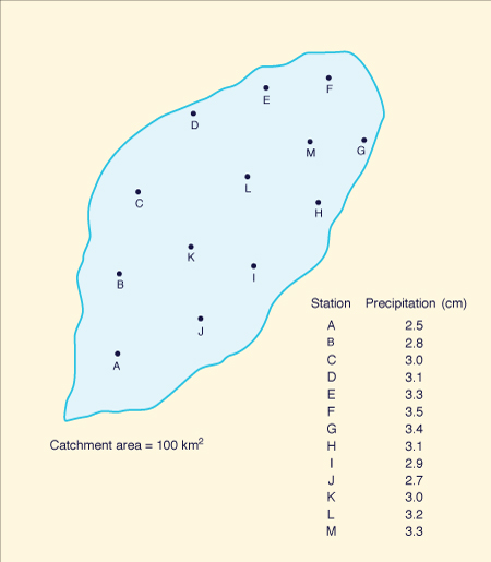
Time (h) 0-3 3-6 6-9 9-12 Rainfall (cm) 0.4 0.8 1.6 0.2
Time (%) 0 10 20 30 40 50 60 70 80 90 100 Rainfall depth (%)
0 5 10 25 50 75 90 95 97 99 100
Intensity (mm/h) 50 30 Duration (h) 0.5 1.0
Intensity (mm/h) 60 40 Duration (h) 1 2
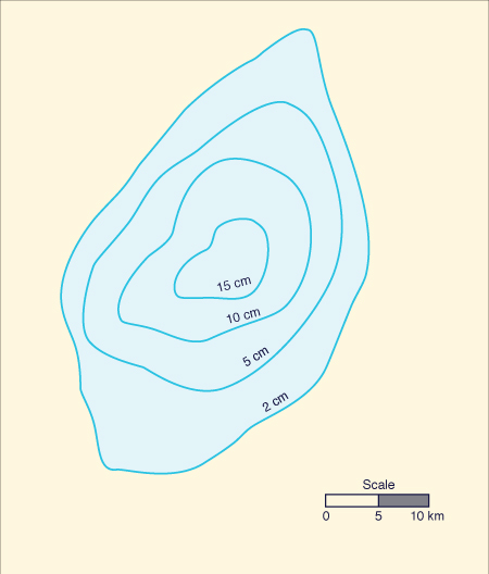
Quadrant) Precipitation
(mm)Distance
(km)I 25 8.5 II 28 6.2 III 27 3.7 IV 30 15.0
Year Precipitation at Z
(mm)10-station average
(mm)1972 35 28 1973 37 29 1974 39 31 1975 35 27 1976 30 25 1977 25 21 1978 20 17 1979 24 21
Year Precipitation at Z
(mm)10-station average
(mm)1980 30 26 1981 31 31 1982 35 36 1983 38 39 1984 40 44 1985 28 32 1986 25 30 1987 21 23
Time
(h) f
(mm/h)1 2.35 3 1.27 ∞ 1.00
Time
(h) f
(mm/h)2 1.7 4 1.5
Time (h) 0-2 2-4 4-6 6-8 8-10 10-12 Rainfall intensity (cm/h)
1.0 2.0 4.0 3.0 0.5 1.5
Jan Feb Mar Apr May
Jun Jul Aug Sep Oct Nov Dec 6
8 10 12 15 20 25
20 16 12 10 8
Elevation
(m)Subarea above
indicated elevation
(km2)1010 135 1020 85 1030 65 1040 30 1050 12 1060 4 1070 0
Distance (km) 0 50 100 150
200 250 300 Elevation (m)
10 30 60 100
150 220 350
Day Precipitation
(cm)1 0.0 2 0.1 3 0.3 4 0.4 5 0.2
Day Precipitation
(cm)6 0.0 7 0.0 8 0.7 9 0.8 10 0.9
Day Precipitation
(cm)11 1.2 12 0.5 13 0.0 14 0.0
Jan Feb Mar Apr May
Jun Jul Aug Sep Oct Nov Dec
30 34 35 48 72 85
72 55 51 40 34 32
http://engineeringhydrology.sdsu.edu
160821 17:50
Documents in Portable Document Format (PDF) require Adobe Acrobat Reader 5.0 or higher to view;
download Adobe Acrobat Reader.