|
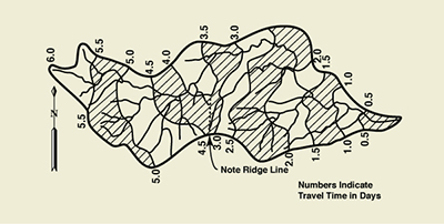
Isochrones for the
Appomattox River at Petersburg, Virginia |
| |
|
|
ABSTRACT
Clark's original unit hydrograph (Clark, 1945) and Ponce's Clark unit
hydrograph (Ponce, 1989) are explained and compared.
Clark's procedure routes, through a linear reservoir, a discrete unit-runoff hyetograph,
while Ponce's procedure routes a continuous unit hydrograph.
Since the unit hydrograph has a longer time base than the unit-runoff hyetograph,
Ponce's procedure provides a longer time lag and, consequently, a correspondingly smaller peak discharge than Clark's original methodology.
The difference, however, does not appear to be substantial.
As expected,
both methods are shown to be 100% mass conservative.
|
1. INTRODUCTION
The Clark unit hydrograph (Clark, 1945)
was included in the original HEC-1 model of the
U.S. Army Corps of Engineers (Hydrologic Engineering Center, 1990).
A variation of the Clark method, referred to as ModClark, forms part of Hydrologic Engineering Center's HEC-HMS, the second generation hydrologic model
of the U.S. Army Corps of Engineers, which superseded HEC-1 in 1998. Despite its
apparent ubiquitousness in Corps literature, details about the Clark model are not
widely available, with a notable exception in Ponce's textbook (1989).
Herein, we endeavor to clarify the origins of the methodology, to explain its theoretical basis,
and to compare: (1) the original 1945 Clark model, with (2) Ponce's 1989 Clark model.
In a nutshell, the Clark unit hydrograph is derived by routing the discrete, time-area-method-derived,
unit-runoff hyetograph
through a linear reservoir. Instead, Ponce's Clark procedure routes the continuous,
time-area-method-derived, unit hydrograph through a linear reservoir.
The storage coefficient K of the linear reservoir is chosen empirically
to provide the appropriate amount of runoff diffusion, i.e.,
the correct time lag and unit hydrograph peak.
2. HEC-HMS CLARK UNIT HYDROGRAPH
The HEC-HMS Clark unit hydrograph requires the specification of the watershed/basin drainage area A,
the time of concentration Tc , the linear reservoir's storage constant K, and the time-area histogram.
If no basin-specific time-area histogram is available, HEC-1 provides a default time-area curve [a two end-to-end parabola-shaped basin] from which
a time-area histogram may be obtained (Kull and Feldman, 1998). In cases where the actual watershed/basin shape deviates substantially from this standard shape, it
is advisable to construct a basin-specific time-area histogram.
The HEC-MHS model's default time-area curve is:
T* = Ti / Tc
A* = Ai / A
A* = 1.414 T*1.5 [ 0 ≤ T* ≤ 0.5 ]
A* = 1 - 1.414 (1 - T*)1.5 [ 0.5 < T* ≤ 1 ] |
(1) | |
where Ti and Ai are cumulative time and cumulative area, respectively.
For example, given A = 1000 km2 and Tc = 6 hr, the calculated default time-area histogram
for this watershed data is shown in Table 1. The time of concentration is conveniently divided into six (6) 1-hr intervals.
Using the default time-area curve (Eq. 1), the watershed area is divided into six (6) corresponding subareas, shown in Col. 4 of Table 1.
The calculated time-area histogram is shown in Fig. 1.
| Table 1. HEC's default time-area histogram for A
= 1,000 km2 and Tc = 6 hr.
|
| [1] |
[2] |
[3] |
[4] |
| Histogram increment i |
Cumulative time Ti at the end of increment i (hr) |
Cumulative area Ai at the end of cumulative time Ti
(km2) |
Incremental area ΔAi
(km2) |
| 1 |
1 |
96.2 |
96.2 |
| 2 |
2 |
272.1 |
175.9 |
| 3 |
3 |
500 |
227.9 |
| 4 |
4 |
727.9 |
227.9 |
| 5 |
5 |
903.8 |
175.9 |
| 6 |
6 |
1,000 |
96.2 |
Fig. 1 Calculated time-area histogram.
3. ROUTING PRINCIPLES
In surface-water hydrology, the term "routing" refers to the calculation of flows in time and space.
The objective is to transform an inflow,
either (a)
an effective precipitation hyetograph in the case of watersheds/basins,
or (b) a streamflow hydrograph in the case of reservoirs and channels,
into an outflow hydrograph.
In general, flow routing embodies two distinct physical processes: - convection, commonly referred to as translation or concentration, and
- diffusion, commonly referred to as attenuation or storage.
Convection is interpreted as the movement of water in a direction parallel to the channel bottom.
Diffusion may be interpreted as the movement of water in a direction perpendicular to the channel bottom.
Mathematically, convection is a first-order process, while diffusion is a second-order process (Ponce, 1989).
Three types of physical features are recognized: - reservoirs,
- stream channels, and
- watersheds/basins.
The behavior of these features with respect to
convection and diffusion varies. Significantly:
In reservoir routing, convection is zero while diffusion is finite; therefore,
reservoir routing lacks convection and produces only diffusion.
In stream channel routing, convection is typically
the dominant process, of first order, while diffusion is usually much smaller, of second order.
For kinematic waves, diffusion is nonexistent;
for diffusion waves, diffusion is relatively small;
for mixed kinematic/dynamic waves, in practice referred to as
dynamic waves, diffusion is large (Ponce and Simons, 1977).
In watershed/basin routing, convection and diffusion are usually
about equal in size and, therefore, they may be
accounted for separately. This is
the basis of the Clark methodology.
The time-area method of watershed routing provides only convection;
in contrast, the linear reservoir routing
method provides only diffusion.
The unit hydrograph is an elemental hydrograph for a given watershed/basin,
subsuming both convection and diffusion in a hydrograph for a unit rainfall impulse.
The Clark unit hydrograph accounts for these two processes separately, first using
the time-area method to provide convection and second,
using the linear reservoir method to provide diffusion.
4. TIME-AREA METHOD
The time-area method of hydrologic watershed/basin routing
transforms an effective storm hyetograph
into a runoff hydrograph (Ponce, 1989).
The method accounts for convection only and does not provide for diffusion.
Therefore, hydrographs calculated with the time-area method show a characteristic lack of diffusion,
resulting in higher peaks and shorter time bases
than those that would have been obtained if diffusion
had been taken into account.
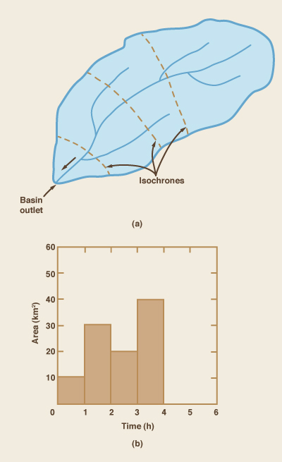
The time-area method is based on the concept of time-area histogram.
To develop a time-area histogram,
the watershed's time of concentration is divided into a number of equal time intervals.
Cumulative time at the end of each time interval is used to divide the watershed into zones delimited by isochrone lines, i.e.,
the loci of points of equal travel time to the outlet. For any point inside the watershed, the travel time
refers to the time that it would take a parcel of water to travel from that point to the outlet. The subareas delimited by the isochrones are measured and plotted in histogram form,
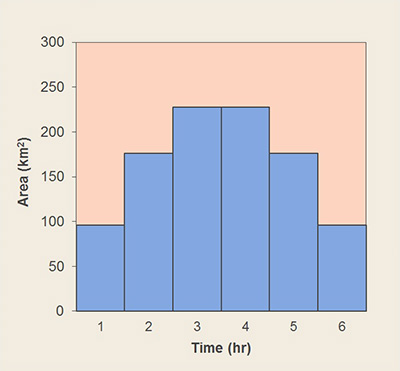
as shown in Fig. 2.
Fig. 2 Time-area method: (a) isochrone delineation; (b) time-area histogram.
For the method to work properly,
the time interval of the time-area histogram (Fig. 2b)
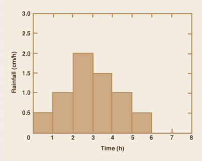
must be the same as that of the effective rainfall hyetograph (Fig. 3). The rationale of the time-area method
is that, according to the runoff concentration principle, the partial flow at the end of each time interval is equal to the product of effective rainfall times the
contributing watershed subarea (Ponce, 1989). The lagging and summation of the partial flows results in a
flood hydrograph corresponding to the given time-area histogram and effective rainfall hyetograph.
Fig. 3 Effective rainfall hyetograph.
Table 2 shows the calculation of the time-area method
using the data of Figs. 2 and 3.
Note that the histogram subareas,
highlighted in red,
are defined for a time interval; for instance,
the value 10 is applicable between time t = 0
to t = 1 hr; 30 between t = 1 to t = 2 hr, and so on.
Also, note the six (6) effective rainfall increments,
highlighted in blue.
| Table 2. Time-area method of watershed/basin routing.
|
| [1] |
[2] |
[3] |
[4] |
[5] |
[6] |
[7] |
[8] |
[9] |
[10] |
Time
(hr) |
Time-area histogram subareas
(km2) |
Partial flows (km2-cm/hr)
for indicated effective rainfall increments |
Outflow
(km2-cm/hr) |
Outflow
(m3/s) |
0.5
cm/hr |
1.0
cm/hr |
2.0
cm/hr |
1.5
cm/hr |
1.0
cm/hr |
0.5
cm/hr |
| 0 |
- |
0 |
- |
- |
- |
- |
- |
0 |
0 |
| 1 |
10 |
5 |
0 |
- |
- |
- |
- |
5 |
13.9 |
| 2 |
30 |
15 |
10 |
0 |
- |
- |
- |
25 |
69.4 |
| 3 |
20 |
10 |
30 |
20 |
0 |
- |
- |
60 |
166.7 |
| 4 |
40 |
20 |
20 |
60 |
15 |
0 |
- |
115 |
319.4 |
| 5 |
- |
0 |
40 |
40 |
45 |
10 |
0 |
135 |
375 |
| 6 |
- |
- |
0 |
80 |
30 |
30 |
5 |
145 |
402.8 |
| 7 |
- |
- |
- |
0 |
60 |
20 |
15 |
95 |
263.9 |
| 8 |
- |
- |
- |
- |
0 |
40 |
10 |
50 |
138.9 |
| 9 |
- |
- |
- |
- |
- |
0 |
20 |
20 |
55.6 |
| 10 |
- |
- |
- |
- |
- |
- |
0 |
0 |
0 |
| Sum |
100 |
- |
- |
- |
- |
- |
- |
650 |
- |
In Table 2, the partial flows for the 0.5 cm/hr rainfall increment are obtained by multiplying each one of the subareas of Col. 2 times 0.5 cm/hr.
Likewise, the partial flows for the 1.0 cm/hr rainfall increment are obtained by multiplying each one of the subareas of Col. 2 times 1.0 cm/hr, and lagged 1 hr,
because the 1.0 cm/hr rainfall increment occurs 1 hr later; and so on. The sum across Cols. 3 to 8, shown in Col. 9, gives the ordinates of the outflow hydrograph
in convenient (km2-cm/hr) units.
Column 10 contains the values of Col. 9, converted to discharge units (m3/s).
Note that the time-area method conserves mass exactly. For this example, the total rainfall is 6.5 cm and the
watershed area is 100 km2. Thus, the total rainfall volume is: 100 × 6.5 = 650 km2-cm.
The sum of the ordinates of the runoff hydrograph (Col. 9) is 650 km2-cm/hr.
These are hourly ordinates; thus, the hydrograph volume is: 650 km2-cm/hr × 1 hr = 650 km2-cm.
Also, note that for this example, the time of concentration is Tc = 4 hr, the storm duration is tr = 6 hr, and the hydrograph time base is Tb = 10 hr.
The following relation holds:
While the time-area method accounts for convection only, it has the distinct advantage that the watershed/basin shape is reflected
in the time-area histogram and, therefore, in the runoff hydrograph.
When warranted, diffusion may be
provided by routing the hydrograph calculated by the time-area method through a linear reservoir
with an appropriate storage constant.
Thus, a complete rainfall-runoff model using
the time-area method and adding diffusion
consists of two steps:
Use of the time-area method to provide pure convection,
i.e., generating a translated-only hydrograph.
Routing of the translated-only hydrograph
through a linear reservoir with an appropriate storage constant,
to provide the desired diffusion effect.
5. LINEAR RESERVOIR ROUTING
The linear reservoir method is a computational procedure that provides diffusion
to an inflow hydrograph. In other words, a hydrograph routed through a linear reservoir
effectively diffuses, that is, it lowers its peak flow while it increases its time base.
The amount of diffusion depends on the value of the storage constant K relative to the time interval Δt.
Values of Δt/K less than 2 provide diffusion;
the lesser the Δt/K, the greater the diffusion.
Values of Δt/K greater than 2 provide negative diffusion,
i.e., hydrograph amplification.
therefore, values of Δt/K greater than 2 are not used in reservoir routing
(Ponce, 1989).
Given inflow I, outflow O, time interval Δt, and reservoir storage constant K,
the general formula for the linear reservoir is:
O2 = C0 I2 + C1 I1 +
C2 O1
C0 = (Δt/K) / [ 2 + (Δt/K) ]
C1 = C0
C2 = [ 2 - (Δt/K) ] / [ 2 + (Δt/K) ] |
(3) |
|
Table 3 shows the routing of the discharge hydrograph obtained with the time-area method (Table 2, Col. 9)
through a linear reservoir of storage constant K = 2 hr, with Δt = 1 hr.
Following Eq. 3, the routing coefficients for this example are:
C0 = 0.2; C1 = 0.2;
C2 = 0.6.
| Table 3.
Routing of a time-area hydrograph through a linear reservoir.
|
| [1] |
[2] |
[3] |
[4] |
[5] |
[6] |
[7] |
Time
(hr) |
Time-area
hydrograph ordinates
(km2-cm/hr) |
Partial flows (Eq. 3)
(km2-cm/hr) |
Outflow from
the linear reservoir
(km2-cm/hr) |
Outflow
(m3/s) |
| C0 I2 |
C1 I1 |
C2 O1 |
| 0 |
0 |
- |
- |
- |
0 |
0 |
| 1 |
5 |
1 |
0 |
0 |
1 |
2.78 |
| 2 |
25 |
5 |
1 |
0.6 |
6.6 |
18.33 |
| 3 |
60 |
12 |
5 |
3.96 |
20.96 |
58.22 |
| 4 |
115 |
23 |
12 |
12.58 |
47.58 |
132.17 |
| 5 |
135 |
27 |
23 |
28.55 |
78.55 |
218.19 |
| 6 |
145 |
29 |
27 |
47.13 |
103.13 |
286.47 |
| 7 |
95 |
19 |
29 |
61.88 |
109.88 |
305.22 |
| 8 |
50 |
10 |
19 |
65.93 |
94.93 |
263.69 |
| 9 |
20 |
4 |
10 |
56.96 |
70.96 |
197.11 |
| 10 |
0 |
0 |
4 |
42.58 |
46.58 |
129.37 |
| 11 |
0 |
0 |
0 |
27.95 |
27.95 |
77.64 |
| 12 |
0 |
0 |
0 |
16.77 |
16.77 |
46.58 |
| 13 |
0 |
0 |
0 |
10.06 |
10.06 |
27.94 |
| 14 |
0 |
0 |
0 |
6.04 |
6.04 |
16.77 |
| 15 |
0 |
0 |
0 |
3.62 |
3.62 |
10.07 |
| 16 |
0 |
0 |
0 |
2.17 |
2.17 |
6.03 |
| 17 |
0 |
0 |
0 |
1.30 |
1.30 |
3.62 |
| 18 |
0 |
0 |
0 |
0.78 |
0.78 |
2.17 |
| 19 |
0 |
0 |
0 |
0.47 |
0.47 |
1.30 |
| 20 |
0 |
0 |
0 |
0.28 |
0.28 |
0.78 |
| 21 |
0 |
0 |
0 |
0.17 |
0.17 |
0.47 |
| 22 |
0 |
0 |
0 |
0.10 |
0.10 |
0.28 |
| 23 |
0 |
0 |
0 |
0.06 |
0.06 |
0.17 |
| 24 |
0 |
0 |
0 |
0.04 |
0.04 |
0.10 |
| 25 |
0 |
0 |
0 |
0.02 |
0.02 |
0.07 |
| 26 |
0 |
0 |
0 |
0.00 |
0.00 |
0.00 |
| Sum |
650 |
- |
- |
- |
650.00 |
- |
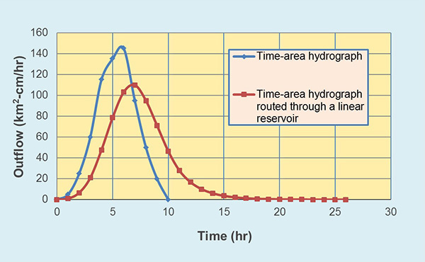
Note that the peak flow has decreased from 145 km2-cm/hr for time t = 6 hr at inflow (Col. 2),
to 109.88 km2-cm/hr for t = 7 hr at outflow (Col. 6).
Also, note that the time base of the hydrograph has increased from 10 hr at inflow, to 26 hr at outflow.
The sum of hydrograph ordinates, 650 km2-cm/hr, is the same at inflow (Col. 2) and outflow (Col.6),
indicating that
routing through the linear reservoir has conserved mass
exactly. Figure 4 shows the effect of routing the time-area hydrograph (Table 2, Col. 9) through a linear reservoir (Table 3, Column 6).
Fig. 4 Effect of routing the time-area hydrograph through a linear reservoir.
6. UNIT HYDROGRAPH CONCEPTS
The unit hydrograph is used in flood hydrology as a means to develop the hydrograph for a given
effective storm hyetograph.
The word "unit" is normally taken to refer to a
unit depth of effective rainfall.
However, the word "unit" also refers to a
unit depth of effective rainfall lasting a "unit" duration, or "unit"
increment
of time, i.e., an indivisible increment (Ponce, 1989). Typical unit hydrograph
durations are
1 hr, 2 hr, 3 hr, 6 hr, 12 hr, and 24 hr. In flood hydrology, unit hydrograph durations from 1 hr to 6 hr are common.
A watersheds/basin can have many unit hydrographs, each for a different duration.
The 1-hr unit hydrograph corresponds to
1 cm [or, alternatively, 1 in] or effective precipitation lasting 1 hr; the 2-hr unit hydrograph corresponds to 1 cm of
effective precipitation lasting 2 hr; and so on. Thus, given a tr -hr unit hydrograph, the effective rainfall
intensity is equal to (1/tr) cm/hr. For a certain basin, once a unit hydrograph for a given duration has been determined,
it may be used to calculate the unit hydrographs for other durations.
A unit hydrograph may be developed from streamgage measurements or by synthetic means.
Once developed, the unit hydrograph contains information on the convection (runoff concentration) and diffusion (runoff diffusion) properties
of the watershed/basin. The unit hydrograph is used as a building block in order to develop the flood hydrograph.
To develop the flood hydrograph, the unit hydrograph is convoluted
with the effective storm hyetograph (Ponce, 1989).
7. CLARK'S ORIGINAL UNIT HYDROGRAPH
Clark (1945) pioneered the use of the time-area method in conjunction
with a linear reservoir as a means
to develop a unit hydrograph.
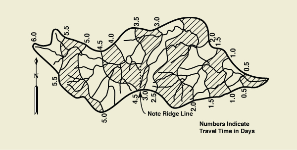
To demonstrate his methodology, Clark used the example of the
Appomattox River at Petersburg, Virginia, with the following data (Fig. 5):
- Drainage area A = 1,335 square miles;
- Time of concentration Tc = 6 days;
- Time interval Δt = 0.5 days = 12 hr;
- Unit hydrograph duration tr = 12 hr;
and
- Linear reservoir storage constant K = 15.428 hr ≅ 15 hr.
Using Eq. 3: C0 = 0.28;
C1 = 0.28;
C2 = 0.44.
Fig. 5 Isochrones for the Appomattox River at Petersburg, Virginia (Clark 1945).
By definition, C1 = C0. Furthermore, within one time step,
Clark used the unit-runoff hyetograph, wherein I2 = I1. Thus, the
linear reservoir routing equation reduces to:
Table 4 shows the computation of the Appomattox River example.
Column 1 shows the time in days. - Column 2 shows the time
in hours.
Column 3 shows the
time-area histogram percentages.
Column 4 shows the incremental areas.
Column 5 shows the inflows, calculated as the areas of Column 4 multiplied by 1 in/hr.
Since the unit hydrograph duration tr = 12 hr,
the rainfall intensity is 1/12 in/hr, each value of Column 5 amounts to 12 times the inflow.
Column 6 is the actual inflow, that is 1/12 of Column 5. Columns 7 and 8 shows the partial flows,
calculated using Eq. 4. Column
9 is the outflow from the linear reservoir, in the routed units (mi2-in/hr).
Column 10 is the outflow (unit hydrograph ordinates), converted to cfs.
The sum of the hydrograph ordinates in Column 9 is 111.249 mi2-in/hr,
which, when integrated over the time interval (12 hr)
and distributed over the basin area (1,335 mi2) results in exactly 1 in of runoff (111.249 × 12 / 1,335 = 1).
Likewise, the sum of the unit hydrograph ordinates in Column 10 is
71,786 cfs, which, when integrated over the
time interval and distributed over the basin area results in exactly 1 in of runoff.
It is important to note that Clark did not route the time-area histogram through a linear reservoir;
indeed one cannot route an area; only a discharge.
Effectively, Clark routed the inflow [unit-runoff hyetograph] shown in Column 5, a value which is linearly related to the area.
To avoid unnecessary complexity, Clark set the
time interval Δt equal to the unit hydrograph duration tr,
thus avoiding the lagging and addition which would have been necessary had
the time interval Δt and unit hydrograph duration tr been different
(See the example of Table 5).
| Table 4.
Calculation of Clark's Appomattox River example.
|
| [1] |
[2] |
[3] |
[4] |
[5] |
[6] |
[7] |
[8] |
[9] |
[10] |
Time
(d) |
Time
(hr) |
Time-area histogram
(%) |
Increment
of area
(mi2) |
12 × Inflow (mi2-in/hr) |
Inflow (mi2-in/hr) |
Partial flows
(mi2-in/hr) |
Outflow (mi2-in/hr) |
Outflow
(UH ordinates)
(cfs) |
| 2 C0 I2 |
C2 O1 |
| 0 |
0 |
- |
- |
- |
- |
- |
- |
0 |
0 |
| 0.5 |
12 |
1.8 |
24.030 |
24.030 |
2.003 |
1.121 |
0.000 |
1.121 |
723.673 |
| 1 |
24 |
3.8 |
50.730 |
50.730 |
4.228 |
2.367 |
0.493 |
2.861 |
1846.170 |
| 1.5 |
36 |
6.9 |
92.115 |
92.115 |
7.676 |
4.299 |
1.259 |
5.557 |
3586.395 |
| 2 |
48 |
10.8 |
144.180 |
144.180 |
12.015 |
6.728 |
2.445 |
9.174 |
5920.052 |
| 2.5 |
60 |
19.1 |
254.985 |
254.985 |
21.429 |
11.899 |
4.036 |
15.936 |
10283.798 |
| 3 |
72 |
7.6 |
101.460 |
101.460 |
8.455 |
4.735 |
7.012 |
11.747 |
7580.380 |
| 3.5 |
84 |
6.5 |
86.775 |
86.775 |
7.231 |
4.050 |
5.168 |
9.218 |
5948.631 |
| 4 |
96 |
5.5 |
73.425 |
73.425 |
6.119 |
3.247 |
4.056 |
7.482 |
4828.621 |
| 4.5 |
108 |
9.0 |
120.150 |
120.150 |
10.013 |
5.607 |
3.292 |
8.899 |
5742.958 |
| 5 |
120 |
14.0 |
186.900 |
186.900 |
15.575 |
8.722 |
3.916 |
12.638 |
8155.470 |
| 5.5 |
132 |
9,5 |
126.825 |
126.825 |
10.569 |
5.919 |
5.561 |
11.479 |
7407.792 |
| 6 |
144 |
5.5 |
73.425 |
73.4250 |
6.119 |
3.427 |
5.051 |
8.477 |
5470.652 |
| 6.5 |
156 |
0 |
0 |
0 |
0 |
0 |
3.730 |
3.730 |
2407.087 |
| 7 |
168 |
0 |
0 |
0 |
0 |
0 |
1.641 |
1.641 |
1059.118 |
| 7.5 |
180 |
0 |
0 |
0 |
0 |
0 |
0.722 |
0.722 |
466.012 |
| 8 |
192 |
0 |
0 |
0 |
0 |
0 |
0.318 |
0.318 |
205.045 |
| 8.5 |
204 |
0 |
0 |
0 |
0 |
0 |
0.140 |
0.140 |
90.220 |
| 9 |
216 |
0 |
0 |
0 |
0 |
0 |
0.062 |
0.062 |
039.697 |
| 9.5 |
228 |
0 |
0 |
0 |
0 |
0 |
0.027 |
0.027 |
17.467 |
| 10 |
240 |
0 |
0 |
0 |
0 |
0 |
0.012 |
0.012 |
7.685 |
| 10.5 |
252 |
0 |
0 |
0 |
0 |
0 |
0.005 |
0.005 |
3.382 |
| 11 |
264 |
0 |
0 |
0 |
0 |
0 |
0.002 |
0.002 |
1.488 |
| 11.5 |
276 |
0 |
0 |
0 |
0 |
0 |
0.001 |
0.001 |
0.655 |
| 12 |
288 |
0 |
0 |
0 |
0 |
0 |
0.00044 |
0.00044 |
0.288 |
| Sum |
- |
100.00 |
1335.000 |
- |
- |
- |
- |
111.249 |
71786.924 |
Table 5 illustrates a more general computation of the Clark procedure,
one where the time interval Δt is not equal to the unit hydrograph duration tr.
For this example, the unit hydrograph duration is tr = 2 hr,
the time interval is Δt = 1 hr, and the linear reservoir storage constant is K = 2 hr.
Following Eq. 3, the routing coefficients are:
C0 = 0.2;
C1 = 0.2; and
C2 = 0.6. To develop the flows,
the histogram subareas are multiplied by two (2) 1-hr rainfall increments of 0.5 cm/hr each, and lagged appropriately.
The sum across Cols. 3 and 4, shown in Column 5, is the discrete unit-runoff hyetograph,
in km2-cm/hr units. The duration of the hyetograph is 5 hr, that is, the sum
of the time of concentration (4 hr) plus the unit hydrograph duration (2 hr) minus 1.
| Table 5.
Calculation of Clark's original unit hydrograph for the case of Δt ≠ tr.
|
| [1] |
[2] |
[3] |
[4] |
[5] |
[6] |
[7] |
[8] |
[9] |
Time
(hr) |
Time-area histogram subareas
(km2) |
Partial flows
for indicated
rainfall increments
(km2-cm/hr) |
Sum
(discrete
unit-runoff
hyetograph)
(km2-cm/hr) |
Partial flows
(Eq. 4)
(km2-cm/hr) |
Outflow from the linear reservoir
(km2-cm/hr) |
Outflow
(m3/s) |
0.5
cm/hr |
0.5
cm/hr |
2 C0 I2 |
C2 O1 |
| 0 |
- |
- |
- |
- |
- |
- |
0 |
0 |
| 1 |
10 |
5 |
- |
5 |
2 |
0 |
2 |
5.56 |
| 2 |
30 |
15 |
5 |
20 |
8 |
1.2 |
9.2 |
25.56 |
| 3 |
20 |
10 |
15 |
25 |
10 |
5.52 |
15.52 |
43.11 |
| 4 |
40 |
20 |
10 |
30 |
12 |
9.31 |
21.31 |
59.19 |
| 5 |
- |
- |
20 |
20 |
8 |
12.79 |
20.79 |
57.75 |
| 6 |
- |
- |
- |
- |
0 |
12.47 |
12.47 |
34.65 |
| 7 |
- |
- |
- |
- |
0 |
7.48 |
7.48 |
20.78 |
| 8 |
- |
- |
- |
- |
0 |
4.49 |
4.49 |
12.47 |
| 9 |
- |
- |
- |
- |
0 |
2.69 |
2.69 |
7.48 |
| 10 |
- |
- |
- |
- |
0 |
1.61 |
1.61 |
4.488 |
| 11 |
- |
- |
- |
- |
0 |
0.97 |
0.97 |
2.688 |
| 12 |
- |
- |
- |
- |
0 |
0.58 |
0.58 |
1.62 |
| 13 |
- |
- |
- |
- |
0 |
0.35 |
0.35 |
0.978 |
| 14 |
- |
- |
- |
- |
0 |
0.21 |
0.21 |
0.58 |
| 15 |
- |
- |
- |
- |
0 |
0.13 |
0.13 |
0.358 |
| 16 |
- |
- |
- |
- |
0 |
0.08 |
0.08 |
0.22 |
| 17 |
- |
- |
- |
- |
0 |
0.05 |
0.05 |
0.13 |
| 18 |
- |
- |
- |
- |
0 |
0.03 |
0.03 |
0.08 |
| 19 |
- |
- |
- |
- |
0 |
0.02 |
0.02 |
0.05 |
| 20 |
- |
- |
- |
- |
0 |
0.01 |
0.01 |
0.03 |
| 21 |
- |
- |
- |
- |
0 |
0.006 |
0.006 |
0.016 |
| 22 |
- |
- |
- |
- |
0 |
0.004 |
0.004 |
0.011 |
| Sum |
100 |
- |
- |
- |
- |
0 |
100.00 |
- |
In Table 5, the discrete unit-runoff hydrograph is highlighted in
cyan color.
Note that Clark's original methodology conserves mass exactly. In effect,
the sum of Column 2 is 100 km2 and the effective rainfall is 1 cm; therefore, the
total rainfall volume is 100 km2-cm. The sum of the hydrograph ordinates in Column 8 is
100 km2-cm/hr, which, when integrated over the time interval Δt = 1 hr,
gives 100 km2-cm.
8. PONCE'S CLARK UNIT HYDROGRAPH
Ponce's Clark unit hydrograph differs slightly from the original Clark procedure.
Ponce applied the time-area method to a given unit rainfall, of intensity 1/tr,
to obtain a continuous
unit hydrograph based on the time-area histogram.
He then routed this unit hydrograph through a linear reservoir to obtain the
Clark unit hydrograph (Ponce, 1989).
Ponce's Clark unit hydrograph retains the essence
of the original methodology, while providing an improved unit hydrograph,
consistent with established routing principles.
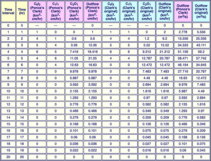
Table 6 illustrates the computation of Ponce's Clark unit hydrograph.
To enable comparison, the data for this example is the same as that of Table 5.
The unit hydrograph duration is tr = 2 hr,
the time interval is Δt = 1 hr, and the linear reservoir storage constant is K = 2 hr.
Following Eq. 3, the routing coefficients are: C0 = 0.2;
C1 = 0.2;
C2 = 0.6. To develop the flows,
the histogram subareas are multiplied by two (2) 1-hr rainfall increments of 0.5 cm/hr each, and lagged appropriately.
The sum across Cols. 3 and 4, shown in Column 5, is the translated-only unit hydrograph, with flow units (km2-cm/hr)
and, following Eq. 2, a time base Tb = 6 hr.
Columns 6, 7, and 8 are the partial flows of the linear reservoir routing.
Column 9 is the sum of Cols. 6, 7, and 8, i.e., the outflow from the linear reservoir.
Column 9 shows that the method conserves mass; the sum of Column 9 is 100.
Note that unlike the discrete unit-runoff hyetograph shown in Column 5 of Table 5,
Column 5 of Table 6 shows a continuous unit hydrograph. That is the difference between the two methods
and that is why the results are slightly different.
Ponce's Clark unit hydrograph has a longer time base (1 hr longer);
consequently, it has a somewhat smaller peak discharge.
| Table 6.
Calculation of Ponce's Clark unit hydrograph.
|
| [1] |
[2] |
[3] |
[4] |
[5] |
[6] |
[7] |
[8] |
[9] |
[10] |
Time
(hr) |
Histogram subareas
(km2) |
Partial flows
for indicated rainfall increments
(km2-cm/hr) |
Sum of Col. 3
and
Col. 4
(translated-only
unit hydrograph)
(km2-cm/hr) |
Partial flows
(Eq. 3)
(km2-cm/hr) |
Outflow from the linear
reservoir
(km2-cm/hr) |
Outflow
(m3/s) |
0.5
cm/hr |
0.5
cm/hr |
C0 I2 |
C1 I1 |
C2 O1 |
| 0 |
- |
- |
- |
0 |
- |
- |
- |
0 |
0 |
| 1 |
10 |
5 |
- |
5 |
1 |
0 |
0 |
1 |
2.78 |
| 2 |
30 |
15 |
5 |
20 |
4 |
1 |
0.6 |
5.6 |
15.55 |
| 3 |
20 |
10 |
15 |
25 |
5 |
4 |
3.36 |
12.36 |
34.33 |
| 4 |
40 |
20 |
10 |
30 |
6 |
5 |
7.42 |
18.42 |
51.17 |
| 5 |
- |
- |
20 |
20 |
4 |
6 |
11.05 |
21.05 |
58.47 |
| 6 |
- |
- |
- |
0 |
0 |
4 |
12.63 |
16.63 |
46.19 |
| 7 |
- |
- |
- |
- |
0 |
0 |
9.98 |
9.98 |
27.72 |
| 8 |
- |
- |
- |
- |
0 |
0 |
5.99 |
5.99 |
16.64 |
| 9 |
- |
- |
- |
- |
0 |
0 |
3.59 |
3.59 |
9.98 |
| 10 |
- |
- |
- |
- |
0 |
0 |
2.15 |
2.15 |
5.98 |
| 11 |
- |
- |
- |
- |
0 |
0 |
1.29 |
1.29 |
3.58 |
| 12 |
- |
- |
- |
- |
0 |
0 |
0.78 |
0.78 |
2.17 |
| 13 |
- |
- |
- |
- |
0 |
0 |
0.47 |
0.47 |
1.30 |
| 14 |
- |
- |
- |
- |
0 |
0 |
0.28 |
0.28 |
0.78 |
| 15 |
- |
- |
- |
- |
0 |
0 |
0.17 |
0.17 |
0.47 |
| 16 |
- |
- |
- |
- |
0 |
0 |
0.10 |
0.10 |
0.28 |
| 17 |
- |
- |
- |
- |
0 |
0 |
0.06 |
0.06 |
0.17 |
| 18 |
- |
- |
- |
- |
0 |
0 |
0.04 |
0.04 |
0.11 |
| 19 |
- |
- |
- |
- |
0 |
0 |
0.02 |
0.02 |
0.06 |
| 20 |
- |
- |
- |
- |
0 |
0 |
0.01 |
0.01 |
0.03 |
| 21 |
- |
- |
- |
- |
0 |
0 |
0.006 |
0.006 |
0.016 |
| 22 |
- |
- |
- |
- |
0 |
0 |
0.004 |
0.004 |
0.011 |
| Sum |
100 |
- |
- |
- |
- |
- |
0 |
100.00 |
- |
In Table 6, the continuous unit hydrograph is highlighted in
magenta color.
Note that Ponce's Clark unit hydrograph conserves mass exactly, as shown by the last lines
of Columns 2 and 8.
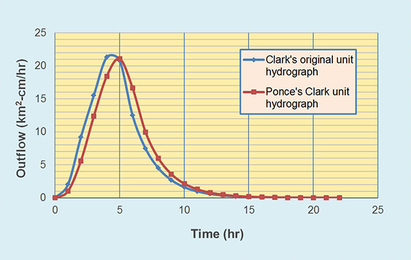
Table 7 shows a side-by-side comparison of the original Clark and Ponce's Clark unit hydrographs.
It is seen that Clark's original unit hydrograph has a somewhat higher peak.
The difference is balanced by the longer tail of Ponce's Clark unit hydrograph.
In addition, Ponce's Clark is lagged about 1 hr to the right, which reflects the time base of the
inflow unit hydrograph (6 hr), as opposed to that of the inflow unit-runoff hyetograph (5 hr).
Both unit hydrographs conserve mass exactly (see bottom line of Cols. 5 and 9).
Figure 6 shows a graphical portrayal of the differences between
the two unit hydrographs.
| Table 7.
Comparison of Clark's original and Ponce's Clark unit hydrographs.
|
| [1] |
[2] |
[3] |
[4] |
[5] |
[6] |
[7] |
[8] |
[9] |
Time
(hr) |
Partial flows
(Eq. 3)
(km2-cm/hr) |
Clark's original
unit hydrograph
(km2-cm/hr) |
Partial flows
(Eq. 3)
(km2-cm/hr) |
Ponce's Clark
unit hydrograph
(km2-cm/hr) |
| C0 I2 |
C1 I1 |
C2 I1 |
C0 I2 |
C1 I1 |
C2 O1 |
| 0 |
- |
- |
- |
0 |
- |
- |
- |
0 |
| 1 |
1 |
1 |
0 |
2 |
1 |
0 |
0 |
1 |
| 2 |
4 |
4 |
1.2 |
9.2 |
4 |
1 |
0.6 |
5.6 |
| 3 |
5 |
5 |
5.52 |
15.52 |
5 |
4 |
3.36 |
12.36 |
| 4 |
6 |
6 |
9.31 |
21.31 |
6 |
5 |
7.42 |
18.42 |
| 5 |
4 |
4 |
12.79 |
20.79 |
4 |
6 |
11.05 |
21.05 |
| 6 |
0 |
0 |
12.47 |
12.47 |
0 |
4 |
12.63 |
16.63 |
| 7 |
0 |
0 |
7.48 |
7.48 |
0 |
0 |
9.98 |
9.98 |
| 8 |
0 |
0 |
4.49 |
4.49 |
0 |
0 |
5.99 |
5.99 |
| 9 |
0 |
0 |
2.69 |
2.69 |
0 |
0 |
3.59 |
3.59 |
| 10 |
0 |
0 |
1.61 |
1.61 |
0 |
0 |
2.15 |
2.15 |
| 11 |
0 |
0 |
0.97 |
0.97 |
0 |
0 |
1.29 |
1.29 |
| 12 |
0 |
0 |
0.58 |
0.58 |
0 |
0 |
0.78 |
0.78 |
| 13 |
0 |
0 |
0.35 |
0.35 |
0 |
0 |
0.47 |
0.47 |
| 14 |
0 |
0 |
0.21 |
0.21 |
0 |
0 |
0.28 |
0.28 |
| 15 |
0 |
0 |
0.13 |
0.13 |
0 |
0 |
0.17 |
0.17 |
| 16 |
0 |
0 |
0.08 |
0.08 |
0 |
0 |
0.10 |
0.10 |
| 17 |
0 |
0 |
0.05 |
0.05 |
0 |
0 |
0.06 |
0.06 |
| 18 |
0 |
0 |
0.03 |
0.03 |
0 |
0 |
0.04 |
0.04 |
| 19 |
0 |
0 |
0.02 |
0.02 |
0 |
0 |
0.02 |
0.02 |
| 20 |
0 |
0 |
0.01 |
0.01 |
0 |
0 |
0.01 |
0.01 |
| 21 |
0 |
0 |
0.006 |
0.006 |
0 |
0 |
0.006 |
0.006 |
| 22 |
0 |
0 |
0.004 |
0.004 |
0 |
0 |
0.004 |
0.004 |
| Sum |
- |
- |
- |
100.00 |
- |
- |
0 |
100.00 |
Fig. 6 Comparison of Clark's original and Ponce's Clark unit hydrographs.
9. ONLINE CALCULATION
The program
ONLINE ROUTING CLARK
enables the calculation and side-by-side comparison of
Clark´s original
and Ponce´s Clark's unit hydrographs.
Figure 7 shows the comparison for the same example shown in Table 7.
Fig. 7 Online calculation of Clark's original and Ponce's Clark unit hydrographs.
10. SUMMARY
Clark's original unit hydrograph (Clark, 1945) and Ponce's
Clark unit hydrograph
(Ponce, 1989) are explained and compared.
Clark's original procedure routes, through a linear reservoir,
the discrete time-area-derived unit-runoff hyetograph (highlighted in
cyan in Table 5),
while Ponce's alternative procedure routes the continuous time-area-derived
unit hydrograph (highlighted in
magenta
in Table 6).
Since the unit hydrograph has a longer time base than the unit-runoff hyetograph,
Ponce's procedure provides a longer time lag
and, consequently, a
correspondingly smaller peak discharge than Clark's original methodology.
The difference, however, does not appear to be substantial.
As expected,
both methods are shown to be 100% mass conservative.
REFERENCES
Clark, C. O., 1945. Storage and the unit hydrograph. Transactions, ASCE, Vol. 110, Paper No. 2261, 1419-1446.
Hydrologic Engineering Center, 1990. HEC-1, Flood Hydrograph Package. Davis, California.
Hydrologic Engineering Center, 2010. HEC-HMS, Hydrologic Modeling System. User's Manual, Version 3.5, August 2010, CDP-74A, Davis, California.
Ponce, V. M., and D. B. Simons. 1977. Shallow wave propagation in open channel flow.
Journal of the Hydraulics Division, ASCE, Vol. 103, No. HY12, December, 1461-1476.
Ponce, V. M. 1980. Linear reservoirs and numerical diffusion. Journal of the Hydraulics Division, ASCE, Vol. 106, No. HY5, May, 691-699.
Ponce, V. M. 1989. Engineering Hydrology: Principles and Practices. Prentice Hall, Englewood Cliffs, New Jersey.
Ponce, V. M. 2009. Cascade and convolution: One and the same. Online article.
|