COMPARISON BETWEEN OVERLAND FLOW MODELS Luis A. Magallón and Victor M. Ponce160322 |

|
Three overland models, ONLINEOVERLAND, SWMM, and HEC-HMS were tested under three cases:
(a) Impervious case, with curve number CN = 100, and total precipitation
The results were analyzed for (1) peak flow, (2) timing of the peak, and (3) mass conservation.
ONLINEOVERLAND behaved properly for the three cases.
Results for peak flow, timing of the peak, and mass conservation were as expected.
SWMM and HEC-HMS behaved more or less properly for the impervious cases (a and c), with some imperfections.
For case b, due to the initial abstraction assumed, SWMM and HEC-HMS showed a peak flow
much higher than expected assuming uniform abstraction.
Given the importance of these models in hydrologic engineering practice, more research is needed to clarify the issues raised in this article.
|
Overland flow is surface runoff that occurs in the form of sheet flow on the land surface without concentrating in clearly defined channels.
This type of flow is the first manifestation of surface runoff, since the latter occurs first as overland flow before it has a chance to flow into channels and become streamflow.
Overland flow theory uses deterministic methods to describe surface runoff in overland flow planes.
The theory is based on established principles of fluid mechanics such as laminar and turbulent flow, mass and momentum conservation, and unsteady free surface flow.
The spatial and temporal description leads to differential equations and to their solution by numerical means.
In this article, we compare three overland flow models:
ONLINEOVERLAND, developed by Dr. Victor Miguel Ponce of San Diego State University, San Diego, California.
SWMM, developed by the U.S. Environmental Protection Agency
HEC-HMS, developed by the Hydrologic Engineering Center, U.S. Army Corps of Engineers, Davis, California.
The models were tested by specifying a common input data set consisting of storm type, catchment characteristics, hydrologic abstraction, and relevant hydraulic parameters.
The catchment is an open book, with runoff from one (or two) plane(s) draining laterally into a (central) channel, the latter draining into the catchment outlet.
Table 1 shows a summary of input data.
Both SI and U.S. Customary units are considered.
ONLINEOVERLAND is a physically based model of overland flow which simulates catchment dynamics using the diffusion wave.
The model requires the input of physical parameters and flow characteristics of both the planes and the channel (Fig. 1).
ONLINEOVERLAND is capable of using SI (metric) or U.S. Customary units, selected at the beginning of data input (Aguilar and Ponce, 2014).
Fig. 1 ONLINEOVERLAND model schematic.
The model has the following components:
The total simulation time Tt and the number of time intervals NΔt determines the time interval Δt.
Once the time interval is determined, the model calculates the space interval such that the Courant number is approximately equal to one, in planes and channel.
The user can enter Npr, the number of time intervals to print.
This is particularly useful for cases in which many calculations are required.
Moreover, the model also requires the input of the fraction used to estimate the reference discharge Fr.
The USDA NRCS runoff curve number method is used to obtain the effective rainfall, or effective runoff depth.
The curve number CN is required input.
For CN = 100, the effective runoff depth is equal to the total rainfall depth.
The effective rainfall depth P is distributed over the duration tr.
The rainfall distribution is specified in three parts:
For instance, for a uniform distribution, the number of points Np = 2; the dimensionless cumulative time T* is the array [0.,1.], and the dimensionless cumulative depth D* is the array [0.,1.].
The model requires a value for the catchment overland flow area A.
The size of each rectangular plane can be determined by specifying the fraction of total area on the left plane Flp and the fraction (of total area) on the right plane Frp.
The slope Sp and the Manning coefficient np for the planes are required inputs.
The rating exponent for the planes βp are required to calculate the Seddon celerity c and
the Vedernikov number V.
The latter is required to determine the hydraulic diffusivity v with dynamic component.
The length of the channel Lch is required for the channel routing component, and the calculation of the width of the planes.
The slope Sch, the Manning coefficient nch, the bottom width Bch, the design depth ych, and the side slope of the channel z [z H : 1 V] are required to calculate the flow velocity.
If the actual flow depth exceeds the specified design depth, a warning error will be produced.
The Muskingum-Cunge method with lateral inflow is used to develop the routing equation for the planes.
Matching physical to numerical diffusivity enables the grid independence of the diffusion wave model.
For the given time interval Δt, the model forces the Courant number
As with the case of the planes, the Muskingum-Cunge method with lateral inflow is used to develop the routing equation for the channel.
As with the routing in the planes, for the given time interval Δt, the model forces the Courant number to be equal to 1.
In the same way as the planes, numerical dispersion is minimized by adjusting the grid ratio such that the Courant number is equal to one.
SWMM was developed in 1971 by the U.S. Environmental Protection Agency, Metcalf and Eddy, Inc. and the Universiy of Florida.
SWMM was originally developed as a model to evaluate combined sewer overflows (CSO) (Roesner, 2013).
It has since undergone major revisions; the current version is Version 5.1.
Fig. 2 SWMM Conceptual Catchment Model.
According to the Applications Manual, SWMM is a distributed model (National Risk Management Research Laboratory, 2009).
This means that the study area may be subdivided into subcatchments, each with its particular characteristics of land cover, length, width, slope, etc.
The subcatchments are modeled as a rectangular surface with a uniform slope, draining into a single channel.
The conceptual model is illustrated in Fig 2.
SWMM has three routing models: (1) Steady flow, (2) Kinematic wave, and (3) Dynamic wave.
The HEC-HMS was developed and is maintained by the Hydrologic Engineering Center, U.S. Army Corps of Engineers.
In contrast to SWMM, which is more suited for urban watersheds, HEC-HMS has been designed to simulate the runoff processes in drainage basins.
Fig. 3 HEC-HMS Conceptual Catchment Model.
In HEC-HMS, the watershed is represented as a series of planes converging into a central channel, as shown in Fig 3.
Surface runoff from the planes is excess rainfall.
Surface runoff to the channel is the lateral inflow from the planes.
Input to each of the models was carried out using the data shown in Table 1.
Typical screenshots are provided in Figs. 4 to 6.
Fig. 4 ONLINEOVERLAND project input display.
Fig. 5 SWMM project input display.
Fig. 6 HEC-HMS project input display.
The models were run under three cases:
Impervious case: CN = 100, with total precipitation
Pervious case: CN = 80, P = 24 cm and, consequently, effective precipitation Pe = 17.7666 cm (Ponce, 2010).
Modified impervious case: CN = 100, and
The outflow hydrographs for this case are shown in Fig. 7.
The following conclusions are drawn:
Peak flow: All three hydrographs reached the expected peak flow, which is equal to:
Qp = I A = (P /tr)A
in which I = effective rainfall intensity, A = watershed area, P = rainfall depth, and tr = total rainfall duration.
For this case:
Qp = (24 cm / 12 hr) × 18 ha × 0.01 m/cm × 10,000 m2/ha / (3600 sec/hr) = 1 m3/s.
Timing of the peak: The three hydrographs showed minor variations in the timing of the peak.
The following observations are made:
ONLINEOVERLAND behaved as expected. The start of the rising limb of
the hydrograph and the start of the receding limb coincided exactly with the start and end of the storm,
respectively.
For SWMM, the start of the rising limb of the hydrograph showed a finite and apreciable lag.
Furthermore, the start of the receding limb began some time after the end of the storm; see Fig. 7.
It is noted that for the impervious case, hydrograph response should start and end at the same time as the precipitation input.
HEC-HMS was slow to rise when compared to the other two models.
Because of this, HEC-HMS was also slow on the tail of the recession; see Fig. 7.
It is noted that for the impervious case, the start of the receding limb should coincide with the end of the precipitation input.
Mass Conservation: The volume V under the hydrograph is:
V = P A
For this case:
V = 24 cm × 18 ha × 0.01 m/cm × 10,000 m2/ha = 43,200 m3
For each model, the calculated hydrograph volume, obtained by Simpson's rule integration, is:
ONLINEOVERLAND: 43,200 m3, which is the same (1.0000) as the expected volume.
SWMM: 43,376 m3, or 1.0041 of the expected volume.
HEC-HMS: 43,305 m3, or 1.0024 of the expected volume.
It is concluded that only ONLINEOVERLAND conserved mass exactly, while SWMM and HEC-HMS failed to conserve mass exactly.
The differences, however, are small and, therefore, they may be neglected on practical grounds.
Fig. 7 Outflow hydrographs for Case A.
The outflow hydrographs for this case are shown in Fig. 8.
The following conclusions are drawn:
Peak flow: The expected peak flow is:
Qp = Ie A = (Pe /tr)A
in which Ie = effective rainfall intensity, A = watershed area, Pe = rainfall depth, and tr = rainfall duration.
For this case:
Qp = (17.7666 cm / 12 hr) × 18 ha × 0.01 m/cm × 10,000 m2/ha / (3600 sec/hr) = 0.740 m3/s.
ONLINEOVERLAND reached the expected peak flow.
However, SWMM and HEC-HMS overshot the expected peak flow based on runoff concentration, with uniform abstraction.
This is due to the fact that both of these models simulate an initial abstraction,
which should be satisfied before runoff starts. In order to conserve mass, the pak flow must exceed the peak flow calculated
based on uniform abstraction.
Timing of the peak: The three hydrographs showed differences in the timing of the peak.
The following observations are made:
ONLINEOVERLAND behaved as expected, assuming constant abstraction.
As with Case A, SWMM showed a finite lag both in the rising limb as well as in the receding limb.
It should be noted that the start of the rising limb should coincide with the end of the storm, which is clearly not the case for SWMM.
HEC-HMS showed a finite lag in the rising limb but not in the receding limb. This last finding is in aggrement with the mechanics of the problem.
Mass Conservation: The volume V under the hydrograph is:
Ve = Pe A
For this case:
Ve = 17.7666 cm × 18 ha × 0.01 m/cm × 10,000 m2/ha = 31,980 m3
For each model, the calculated hydrograph volume, obtained by Simpson's rule integration, is:
ONLINEOVERLAND: 31,979 m3, or 0.99997 (≅ 1.0) of the expected volume.
SWMM: 32,084 m3, or 1.0033 times the expected volume.
HEC-HMS: 31,749 m3, or 0.9928 times the expected volume.
It is concluded that only ONLINEOVERLAND conserved mass exactly, while SWMM and HEC-HMS failed to conserve mass exactly.
The differences, however, are small and, therefore, they may be neglected on practical grounds.
Fig. 8 Outflow Hydrographs for Case B.
The outflow hydrographs for this case are shown in Fig. 9.
The following conclusions are drawn:
Peak flow: All three hydrographs reached the expected peak flow, which is equal to:
Qp = I A = (P /tr)A
in which I = total rainfall intensity, A = watershed area, P = rainfall depth, and tr = total rainfall duration.
For this case:
Qp = (17.7666 cm / 12 hr) × 18 ha × 0.01 m/cm × 10,000 m2/ha / (3600 sec/hr)
Qp = 0.740 m3/s.
Timing of the peak: The three hydrographs showed minor variations in the timing of the peak.
The following observations are made:
ONLINEOVERLAND behaved as expected. The start of the rising limb of
the hydrograph and the start of the receding limb coincided exactly with the start and end of the storm,
respectively.
For SWMM, the start of the rising limb of the hydrograph showed a finite and apreciable lag.
Furthermore, the start of the receding limb began some time after the end of the storm; see Fig. 7.
It is noted that for the impervious case, hydrograph response should start and end at the same time as the precipitation input.
HEC-HMS was slow to rise;
because of this, it was also slow on the tail of the recession; see Fig. 9.
Mass Conservation: The volume V under the hydrograph is:
V = P A
For this case:
V = 17.7666 cm × 18 ha × 0.01 m/cm × 10,000 m2/ha = 31,980 m3
For each model, the calculated hydrograph volume, obtained by Simpson's rule integration, is:
ONLINEOVERLAND: 31,979 m3, or 0.99997 (≅ 1.0) of the expected volume.
SWMM: 32,094 m3, or 1.0036 of the expected volume.
HEC-HMS: 31,809 m3, or 0.9947 of the expected volume.
It is concluded that only ONLINEOVERLAND conserved mass exactly, while SWMM and HEC-HMS failed to conserve mass exactly.
The differences are small and, therefore, they may be neglected on practical grounds.
Fig. 9 Outflow Hydrographs for Case C.
Table 2 summarizes the results of peak flows for all three runs.
The following conclusions are drawn:
For Case A, all three models reached the expected peak flow (1 m3/s).
For Case B, SWMM and HEC-HMS overshot the expected peak flow. This is due to the fact that these models
simulate an initial asbtraction.
For Case C, all three models reached the expected peak flow (0.74 m3/s).
Table 3 summarizes the results of mass conservation for all three runs. The following conclusions are drawn:
ONLINEOVERLAND conserves mass exactly.
SWMM and HEC-HMS do not conserve the mass exactly, although the error is not significant.
Three overland models, ONLINEOVERLAND, SWMM, and HEC-HMS were tested by specifying a common input data set consisting of storm type, catchment characteristics, hydrologic abstraction, and relevant hydraulic parameters.
The models were run under three cases:
Impervious case, with curve number CN = 100 and total precipitation
Pervious case, with CN = 80, P = 24 cm and, therefore, effective precipitation Pe = 17.7666 cm.
Modified impervious case, with CN = 100 and
The following conclusions are drawn from this study:
ONLINEOVERLAND behaved properly for the three cases (a, b, and c).
Results for peak flow, timing of the peak, and mass conservation were as expected.
SWMM and HEC-HMS behaved more or less adequately for the impervious cases (a and c).
Some inconsistencies were noted in reference to the timing of the peak and percentage mass conservation.
For the pervious case (b), the peak flow exceeded the theoretical value derived assuming constant abstraction.
This is due to the fact that both models assume a finite initial abstraction,
which causes an increase in the peak flow.
It is worth to mention that the initial abstraction in the runoff curve number method is valid for the entire storm.
The purpose of the initial abstraction is to increase the total abstraction beyond that which would be possible without initial abstraction
(Ponce and Hawkins, 1996; Ponce, 2000). It is not well defined if the initial asbtraction should be applied, in a distributed fashion,
to a fractional time at the beginning of the storm. The demonstrated differences between SWMM and HEC-HMS
are attributed to the different models formulations, including initial abstraction.
The results of this study reveal certain inconsistencies in the formulation of the SWMM and HEC-HMS models,
particularly in the timing of the peak.
Given the importance of these models in hydrologic engineering practice, additional research is needed to clarify the issues raised in this article.
REFERENCES
Aguilar, R. D., y V. M. Ponce, 2014.
Onlineoverland: Overland flow using the diffusion wave method. Online program.
Huber, W., and L. Roesner. 2012. "The History and Evolution of the EPA SWMM." Fifty Years of Watershed Modeling - Past, Present, and Future." Boulder, Colorado, September 24-26.
National Risk Management Research Laboratory. 2009. "Stormwater Management Model." Application Manual, United States Environmental Protection Agency, July.
Ponce, V. M. 1986. Diffusion wave modeling of catchment dynamics. Journal of Hydraulic Engineering, Vol. 112, No. 8, August, 716-727.
Ponce, V. M., and R. H. Hawkins. 1996. Runoff curve number: Has it reached maturity?
Journal of Hydrologic Engineering, Vol. 1, No. 1, January, 11-19.
Ponce, V. M. 2000. Notes of my conversation with Vic Mockus. Online article.
Ponce, V. M. 2010.
Onlinecurvenumber: Runoff based on NRCS runoff curve number. Online program.
Ponce, V. M. 2014. Engineering Hydrology, Principles and Practices. Online edition.
U.S. Army Corps of Engineers. 2000. Hydrologic Model System HEC-HMS, Technical Reference Manual. Hydrologic Engineering Center, Davis, California.
Table 1. Input data for overland flow models.
Description
SI
U.S. Customary
Rainfall depth P
24 cm
9.45 in
Runoff curve number CN
Varies
Total rainfall duration tr
12 hr
Number of points in cumulative rainfall distribution Np
2
Dimensionless cumulative time for rainfall distribution T*
0, 1
Dimensionless cumulative depth for rainfall distribution D*
0, 1
Total simulation time Tt
48 hr
Number of time intervals NΔt
96
Number of time intervals for printing Npr
1
Fraction used to estimate reference discharge Fr
0.5
Overland flow area A
18 ha
44.46 ac
Fraction of area in left plane Flp
0.5
Slope of left plane Slp
0.001
Manning coefficient for left plane nlp
0.1
Rating exponent for left plane βlp
2
Slope of right plane Slp
0.001
Manning coefficient for right plane nlp
0.1
Rating exponent for right plane βlp
2
Length of channel Lch
400 m
1312 ft
Slope of channel Sch
0.01
Manning coefficient of channel nch
0.015
Bottom width of channel Bch
2 m
6.56 ft
Design depth of channel ych
0.6 m
1.968 ft
Side slope of channel z [z H :1 V]
3
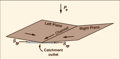
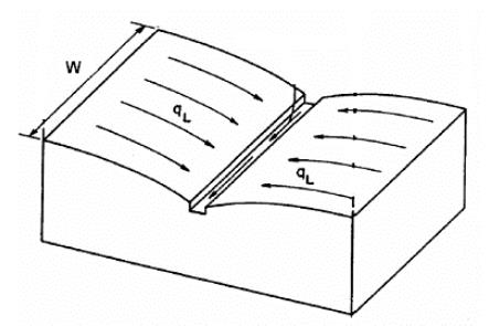
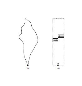
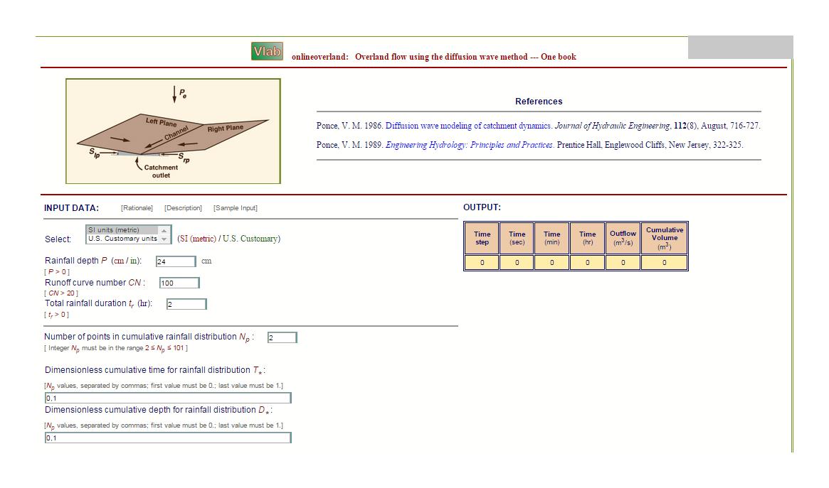
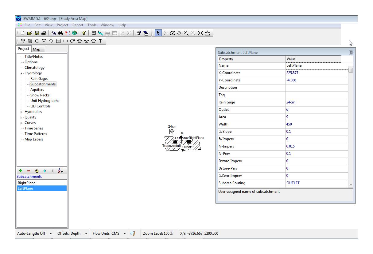
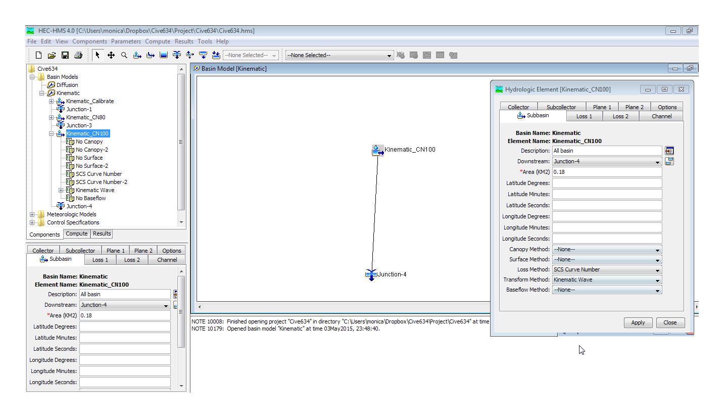
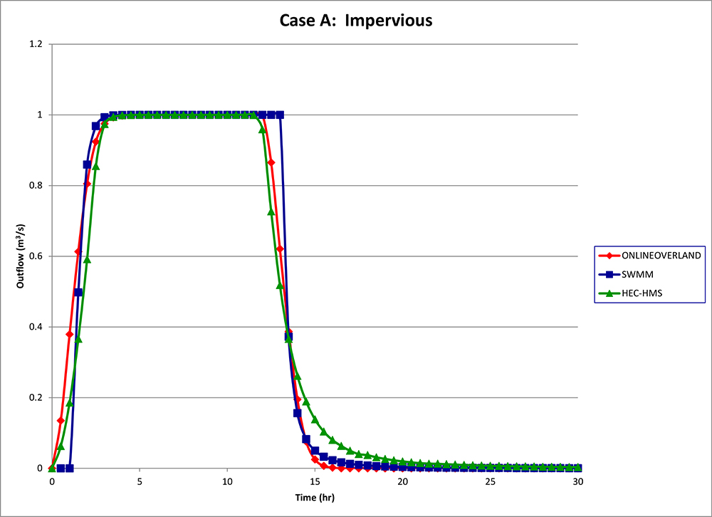
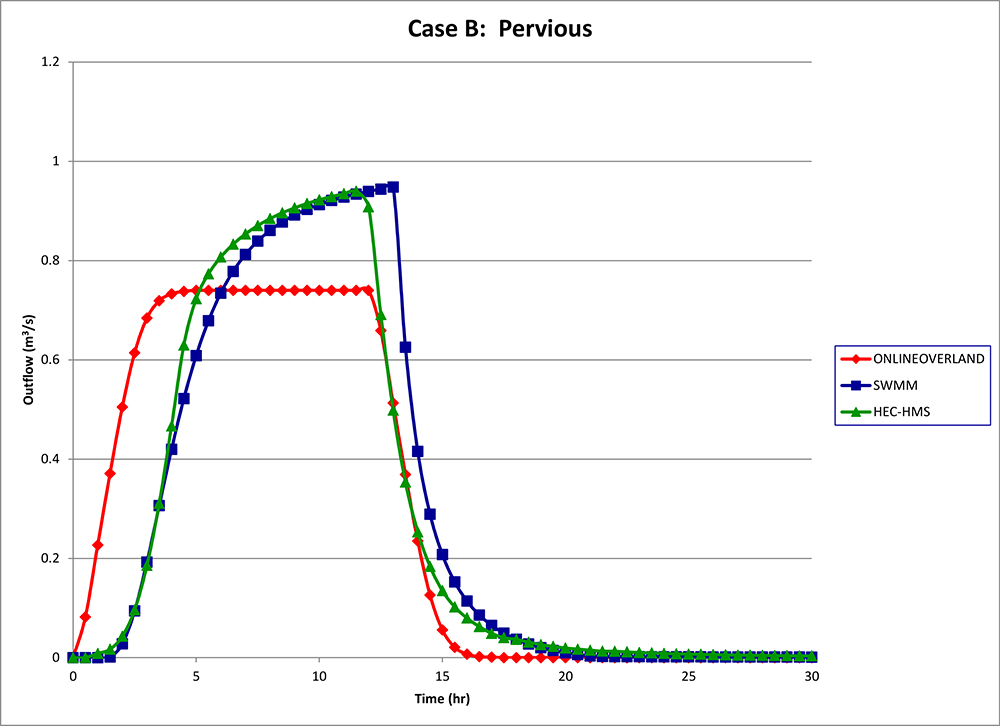
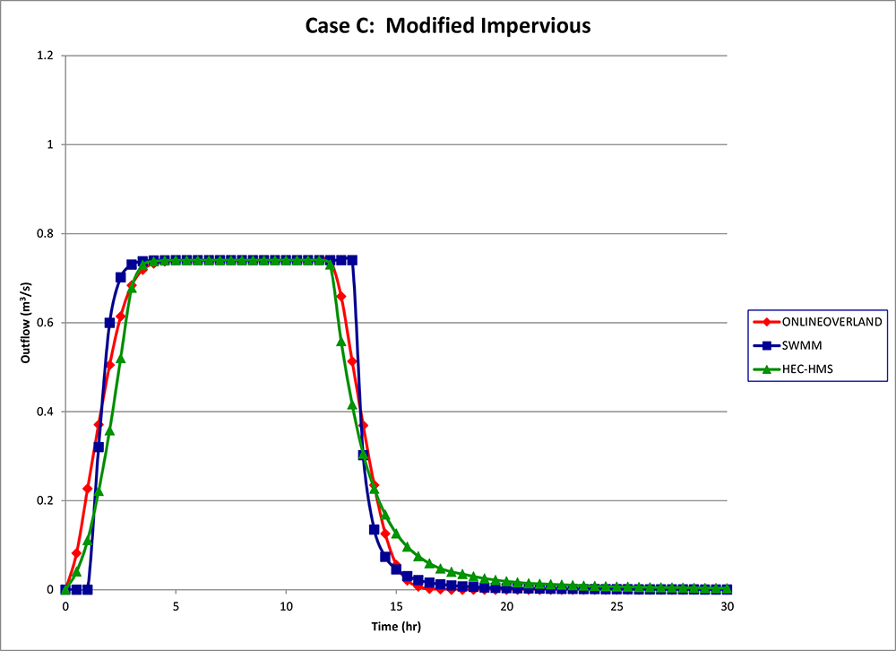
Table 2. Calculated peak flows.
Case
Description
CN
Effective precipitation (cm)
Expected peak flow (m3/s)
Calculated peak flow (m3/s) ONLINE OVERLAND
SWMM
HEC-HMS
A
Impervious
100
24.0000
1.0000
1.0000
1.0000
1.0000
B
Pervious
80
17.7666
0.7400
0.7400
0.9480
0.9396
C
Modified Impervious
100
17.7666
0.7400
0.7400
0.7400
0.7400
Table 3. Results of mass conservation.
Case
Description
CN
Effective precipitation (cm)
Effective volume
(m3)Calculated volume/Effective volume ONLINE OVERLAND
SWMM
HEC-HMS
A
Impervious
100
24.0000
43,200
1.00000
1.0041
1.0024
B
Pervious
80
17.7666
31,980
0.99997
1.0033
1.0028
C
Modified Impervious
100
17.7666
31,980
0.99997
1.0036
0.9947