FINAL DRAFT [080828a] Evolution of sand mining pits in alluvial rivers Vittorio Bovolin University of Salerno, Salerno, Italy Victor Miguel Ponce San Diego State University, San Diego, California Introduction Sand and gravel are widely used as construction materials. Main sources of 'natural' sand and gravel are from alluvial deposits, while 'artificial' sand and gravel come from crushing rocks or boulders. The quality of sediments is one of the key factors driving the choice of mining technology that is applied in each particular case. For example, gravel tends to be rounded with smooth edges, while crushed stone tends to have sharp edges. Generally speaking, the construction industry prefers round sediments to sharps ones. Higher quality, easier accesibility and lower "direct" costs lead to a preference for natural aggregates as opposed to artificial ones. Natural sand and gravel are extracted from glacial deposits, alluvial fans, marine terraces, and river and stream terraces, floodplains, and channels. Sand and gravel can be extracted in various ways. The method chosen at each location depends on many factors, among them, the nature of the deposits, the operator preference, and the amount of materials that are going to be mined. In alluvial rivers, sand and gravel mining may be accomplished as near-stream mining or in-stream mining (Larger 1990). Near-stream mining is carrying out mining in a wide channel that stays dry at low stages, while only a narrow channel is left for conveying the discharge; at high stages the whole area is flooded. In some parts in-stream mining is the only locally available option for aggregate resources. In-stream mining operations range from floating operations on large rivers using specifically equipped barges to small land-based operations on small streams that excavate using a backhoe. Possible in-stream mining methods are: using a floating barge equipped with a hydraulic dredge; using conventional earth moving equipment; using draglines. Channels are dynamic systems that respond rapidly to outside stimuli such as aggregate extraction. The response may affect the hydraulic characteristics and water quality. Effects include increased turbidity, reduced light penetration, increased temperature, and resuspension of organic or toxic materials which may affect aquatic habitat, including spawning beds, and nursery, shellfish, and riparian habitat. Hydraulic impacts may include: Channel modifications such as widening or deepening the channel, creation of deep pools, loss of riffles, alteration of bedload, alteration of channel flow, and degraded aesthetics; Upstream and downstream erosion, and related impacts to bridges and other infrastructure whose foundations may be undermined by the lowering of the riverbed. One particular aspect of the problem that deserves increased attention is the conditions under which the mining pit will affect only the river reach downstream of the pit, and when it will also affect the upstream reach. In this regard, Ponce et al (1979a,b) have established that under unsteady one-dimensional flow, small disturbances travel downstream in the case of subcritical flows and upstream for supercritical flows. There are many references in the literature confirming the downstream movements of 'trenches' or 'holes' (van Rjin 1986, Lee 1993, Ponce 1983). However, there are also many papers reporting the upstream migration of the nickpoint of a sand or gravel mining 'pit' (Collins and Dunne 1990, Kondolf 1994a, Kondolf 1994b, Sandecki and Avila 1997, Surian and Rinaldi 2003). The use of names such as 'holes' or 'pits' may reflect the fact that they are referring to somewhat different morphological conditions. While one-dimensional theory supports the view that the disturbance moves downstream under subcritical flow, there is sufficient empirical evidence to justify the argument in favor of some type of upstream erosion. To clarify this issue, we use herein a model based on the numerical integration of the Saint Venant, Exner, and sediment transport equations. This software (SRH-1D v. 2.0.5) is distributed free-of-charge by the U.S. Bureau of Reclamation (Huang and Greimann, 2007). Theoretical background Ponce et al. (1979a, 1979b) and Ponce (1982) studied analytically the set of equations composed by the Saint Venant, Exner, and sediment transport equations, in relation to the evolution of alluvial channel beds. The disturbance celerity was expressed as a function of several hydraulic and sediment transport parameters, including flow velocity, Froude number, and length of the disturbance. Ponce assumed that the unit-width sediment transport rate could be modeled as a power function of the form: Following linear stability analysis, the disturbance celerity has the following form: in which uo is the uniform flow velocity; cad is the nondimensional celerity: and φ is a sediment transport parameter: in which p is the porosity, and ρs is the specific gravity of the sediments. Numerical simulation of the evolution of small disturbances The following was assumed in order to carry out the numerical simulations: the river may be considered hydraulically wide; the flow is subcritical (Fr<0.95); The flow conditions are uniform throughout the study reach, except at the vicinity of the 'pit'. Calculations have been performed with a constant discharge. The hydraulic boundary conditions have been set according to the type of flow simulated: upstream discharge and downstream depth for subcritical flows, and upstream equilibrium for the sediment transport. The latter condition is appropriate as long as the upstream model limit is not reached by any downstream disturbance. Twenty-eight (28) simulations were run. Details of the simulations are given in Table 1. Table 1. Hydraulic parameters for model testing. N Discharge Length Depth - (m2/s) (m) (m) 1 1.25 1000 0.025 2 1.25 1000 0.050 3 1.25 1000 0.150 4 1.25 1000 0.300 5 1.25 1000 0.600 6 1.25 1000 1.000 7 1.25 1000 2.000 8 1.25 2500 0.025 9 1.25 2500 0.050 10 1.25 2500 0.150 11 1.25 2500 0.300 12 1.25 2500 0.600 13 1.25 2500 1.000 14 1.25 2500 2.000 15 2.50 1000 0.025 16 2.50 1000 0.050 17 2.50 1000 0.150 18 2.50 1000 0.300 19 2.50 1000 0.600 20 2.50 1000 1.000 21 2.50 1000 2.000 22 2.50 2500 0.025 23 2.50 2500 0.050 24 2.50 2500 0.150 25 2.50 2500 0.300 26 2.50 2500 0.600 27 2.50 2500 1.000 28 2.50 2500 2.000 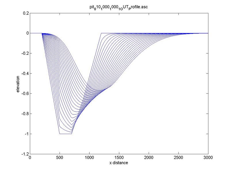Figure 1 depicts a typical riverbed profile evolution for a small initial disturbance. The downstream migration is evident. Fig. 1   Typical riverbed profile evolution for a small initial disturbance. 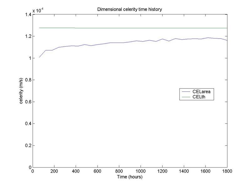Based on the results shown in Fig. 1, the celerity of the disturbance was calculated in the following manner. At each time step, the centroid of the area comprising the disturbance was determined. For each run, the celerity of the disturbance calculated with the numerical model was compared with the theoretical value. A typical comparison is shown in Figure 2. Fig. 2   Time history of celerity for a small disturbance. As shown in Fig. 2, celerity increases in time and asymptotically approaches the theoretical value. This is attributed to the gradual decrease of the disturbance depth. 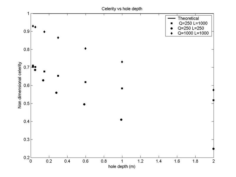In order to compare celerities corresponding to different discharges, calculated values were nondimensionalized by dividing each value by its corresponding theoretical value. The results are depicted in Fig. 3. Fig. 3   Nondimensional celerity vs. initial disturbance depth. Figure 3 shows the following consistent trend: as the disturbance gets smaller, compared to the flow depth, the celerity gets closer to the theoretical value. This confirms the ability of the model to approximately reproduce the analytically determined values. Theoretical analysis of the evolution of large disturbances The remainder of this paper deals with the morphological evolution of large disturbances such as the ones resembling sediment mining pits. The specific objective is to explain what has been observed in real cases, and to provide a practical way to distinguish between cases for which upstream migration may be taking place, from cases where it is not. Firstly, a theorethical analysis of the flow occurring along mining pits is accomplished. Secondly, the results of numerical calculations simulating realistic-scale cases are reported. Results obtained with the numerical model are shown to be in full agreement with the theory. 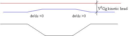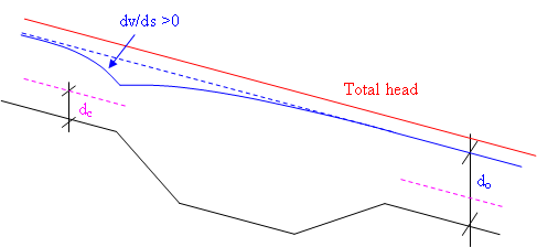There are two contrasting effects where the flow depth increases: a reduction in kinetic head and a reduction in energy slope. The first effect increases the water level, while the second decrease it. Because the reduction in kinetic head is local, while the reduction in energy slope is cumulative in space, it is the length of the pit that decides which effect will prevail. The order of magnitude of these effects may be assessed according to the following analysis. We define a 'short' pit when the effect due to the reduction of the friction losses is negligible compared to one induced by the change in velocity head. Figure 4 contains a conceptual sketch of flow along a 'short pit'. Fig. 4   Conceptual sketch for 'short' pit. We define a 'long' pit when the effect due to the reduction of friction losses is larger than that due to the change in velocity head. Figure 5 contains a conceptual sketch of flow along a 'long' pit. Fig. 5   Conceptual sketch for 'long' pit. With reference to Fig. 4, as the velocity decreases upstream, the flow depth increases and the water surface gets closer to the total head. The order of magnitude of the water surface increase may be assumed of the same order of magnitude as the kinetic head V2/(2g). Since the order of magnitude of velocity may be estimated as Therefore, the order of magnitude of kinetic head is The amount of water surface lowering below the normal depth level may be assumed to be of the order of magnitude of the term SoL (Ponce et al 1979 a, 1979b). Equating the two terms above leads to the following expression: , which allows to estimate the limiting length L1 characterizing a short pit. Values obtained from this expression are reported in Table 2. Table 2. Limiting length for 'short' pit. yn Manning's n 0.033 0.067 0.100 1 47 11 5 2 118 29 13 3 203 49 22 4 297 72 32 5 400 97 44 6 510 124 56 7 627 152 68 8 749 182 82 9 876 213 95 10 1008 245 110 We define a pit 'short' when the pit's length L is shorter than the limiting length L1, while the pit is considered 'long' if the pit's length L is longer than the limiting length L1. With reference to Fig. 4, it may observed that for a short pit the water profile in the reach of river upstream the pit is not affected by the presence of the pit itself and, therefore, there is no change in the bed elevation. With reference to Fig. 5, the lowering of the water surface that takes place along the pit modifies the boundary condition at the end of the upstream reach and brings about an M2 profile, which leads to bed erosion moving progressively upstream. Results contained in Table 2 explain the case of marine trenches, which have been extensively studied. In this case, where the sea bottom is practically flat and the water depth large, it has been observed that trench migration is in the direction of the current. Examples of physical and numerical research carried out on short pits can be found in the literature. Alfrink and van Rijn (1983) carried out numerical simulations, while Lee et al (1993) performed physical experiments. In the case of the Alfrink and van Rjin (1983) runs, the depth was 0.39 m, which implies that for the limiting length to be equal to the pit length (of 6.0 m), the Manning coefficient should be larger than 0.05. In the case of Lee et al (1993), which had a minimum depth of 0.069 m and a pit length of 0.54 m, the Manning coefficient should also have been larger than 0.05. For alluvial rivers, the limiting length provides a ready way to determine morphological parameters that allows classification of a pit as 'long' or 'short', and, therefore, to predict its morphological evolution. Numerical simulation of the evolution of large disturbances A total of 64 simulations for three slopes have been run; 12 simulations each for slopes of 0.00010 and 0.00025, and 40 simulations for the slope of 0.00050. Details of the simulations are given in Table 3. Table 3.   Summary of simulations. N Slope Discharge Length Depth - (m/m) (m2/s) (m) (m) 1 0.00010 1.25 1000 1.00 2 0.00010 1.25 1000 2.00 3 0.00010 1.25 2500 1.00 4 0.00010 2.50 1000 1.00 5 0.00010 2.50 1000 2.00 6 0.00010 2.50 2500 1.00 7 0.00010 5.00 1000 1.00 8 0.00010 5.00 1000 2.00 9 0.00010 5.00 2500 1.00 10 0.00010 10.00 1000 1.00 11 0.00010 10.00 1000 2.00 12 0.00010 10.00 2500 1.00 13 0.00025 1.25 1000 1.00 14 0.00025 1.25 1000 2.00 15 0.00025 1.25 2500 1.00 16 0.00025 2.50 1000 1.00 17 0.00025 2.50 1000 2.00 18 0.00025 2.50 2500 1.00 19 0.00025 5.00 1000 1.00 20 0.00025 5.00 1000 2.00 21 0.00025 5.00 2500 1.00 22 0.00025 10.00 1000 1.00 23 0.00025 10.00 1000 2.00 24 0.00025 10.00 2500 1.00 25 0.00050 1.25 100 1.00 26 0.00050 1.25 250 1.00 27 0.00050 1.25 500 1.00 28 0.00050 1.25 1000 0.50 29 0.00050 1.25 1000 1.00 30 0.00050 1.25 1000 2.00 31 0.00050 1.25 1000 3.00 32 0.00050 1.25 1000 4.50 33 0.00050 1.25 2500 1.00 34 0.00050 1.25 5000 1.00 35 0.00050 2.50 100 1.00 36 0.00050 2.50 250 1.00 37 0.00050 2.50 500 1.00 38 0.00050 2.50 1000 0.50 39 0.00050 2.50 1000 1.00 40 0.00050 2.50 1000 2.00 41 0.00050 2.50 1000 3.00 42 0.00050 2.50 1000 4.50 43 0.00050 2.50 2500 1.00 44 0.00050 2.50 5000 1.00 45 0.00050 5.00 100 1.00 46 0.00050 5.00 250 1.00 47 0.00050 5.00 500 1.00 48 0.00050 5.00 1000 0.50 49 0.00050 5.00 1000 1.00 50 0.00050 5.00 1000 2.00 51 0.00050 5.00 1000 3.00 52 0.00050 5.00 1000 4.50 53 0.00050 5.00 2500 1.00 54 0.00050 5.00 5000 1.00 55 0.00050 10.00 100 1.00 56 0.00050 10.00 250 1.00 57 0.00050 10.00 500 1.00 58 0.00050 10.00 1000 0.50 59 0.00050 10.00 1000 1.00 60 0.00050 10.00 1000 2.00 61 0.00050 10.00 1000 3.00 62 0.00050 10.00 1000 4.50 63 0.00050 10.00 2500 1.00 64 0.00050 10.00 5000 1.00 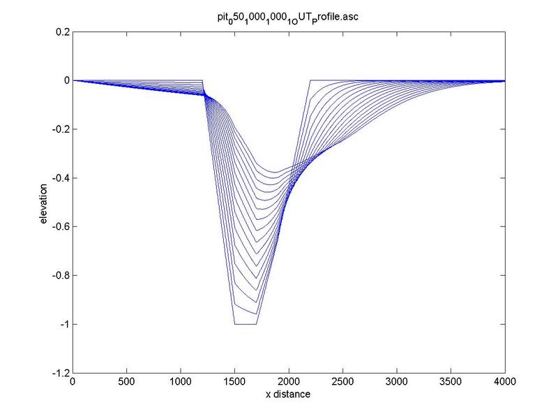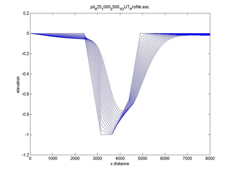A typical example of evolution of water and bed profile in a pit is shown in Figure 6 . Fig. 6   Typical bed and water surface profile for 'long pit'. For the sake of clarity, the bottom bed profile has been taken as a reference line for all simulations. In the case of a long pit, there are two distinct processes: (1) the erosion of the upstream portion, where the bottom profile tends to be linear, and (2) the erosion of the downstream portion, where the disturbance is traveling downstream. 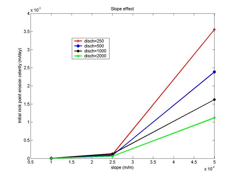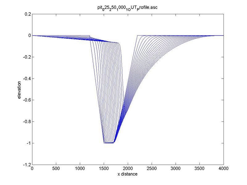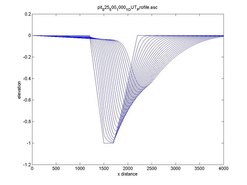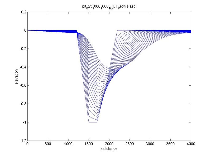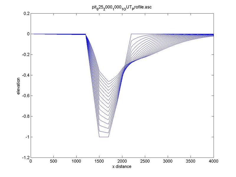Effect of river slope Typical bed-profile evolution at increasing slope is depicted in Fig. 7. Fig. 7.   Typical bed-profile evolution at increasing slope (a) 0.00010 m/m, (b) 0.00025 m/m, (c) 0.00050 m/m. Figure 8 contains the curves concerning the initial rate of erosion calculated at the upstream nickpoint vs slope. Fig. 8   Initial rate of erosion at the upstream nickpoint vs slope. Figure 8 shows that increasing river slope increases the initial erosion rate that takes place at the upstream nickpoint. Effect of increasing discharge The effect of increasing pit discharge is depicted in Fig. 9, where the time-history profile evolution at the same time steps is reported. Fig. 9   Bed profile evolution at increasing discharge: (a) 1.25 m2/s, (b) 2.50 m2/s, (c) 5.00 m2/s, (d) 10.00 m2/s. 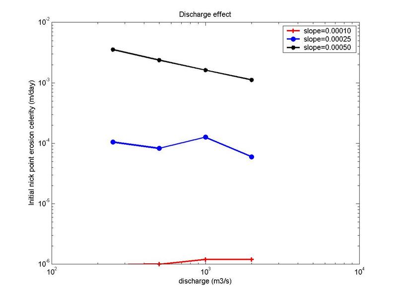Figure 10 contains the curves concerning the initial rate of erosion calculated at the upstream nickpoint vs discharge. Fig. 10   Initial rate of erosion at the upstream nickpoint vs discharge. Figure 10 shows that increased discharge reduces the initial rate of erosion that takes place at the upstream nickpoint. 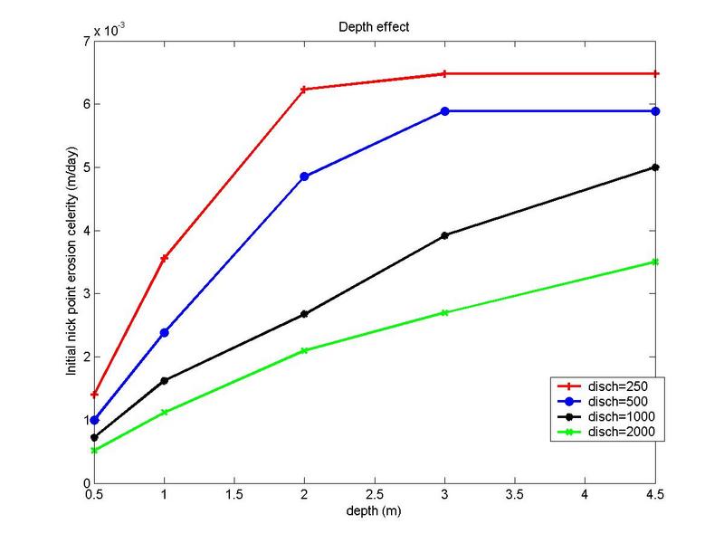Effect of pit depth The effect of increasing pit depth is depicted in Fig. 11, where the time history of profile evolution at the same time step is reported. Fig. 11   Bed-profile evolution at increasing depth: (a) D = 1 m, (b) D = 2 m. Figure 12 contains the curves concerning the initial rate of erosion calculated at the upstream nickpoint vs. pit depth. Fig. 12   Initial rate of erosion at the upstream nickpoint vs depth. Figure 12 shows that above a certain value, the increase in pit depth does not affect the initial rate of erosion that takes place at the upstream nickpoint. 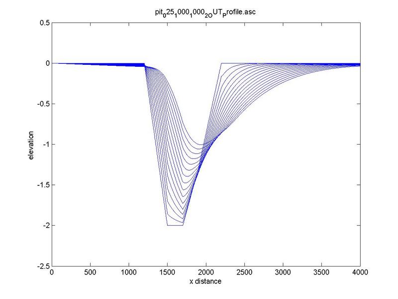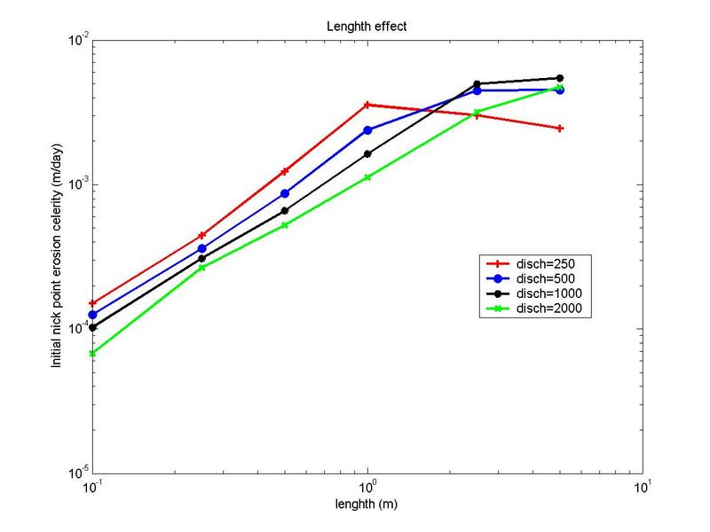Effect of pit length The effect of increasing pit length is depicted in Fig. 13, where the time history of profile evolution at the same time step is reported. Fig. 13   Bed-profile evolution at increasing length: (a) L=1000 m, (b) L=2500 m. Figure 13 shows that increasing length at constant discharge leads to increasing upstream erosion. Fig. 14   Initial rate of erosion at the upstream nickpoint vs pit length. Figure 14 shows that above a certain value, the increase in pit length does not affect the initial rate of the erosion that takes place at the upstream nickpoint. Effect of stream power It may be concluded that in most cases, the depth and length do not substantially influence the erosion process that is taking place upstream. In Fig. 15, the average celerity of the upstream disturbance is plotted vs stream power (SQ). The latter parameter correlates very well with the average celerity. Fig. 15   Initial rate of erosion at the upstream nickpoint vs stream power. Conclusions The analysis reported herein confirms that there are two effects governing borrow pit evolution. The primary effect is downstream in subcritical flow. This effect consists on the propagation of the disturbance at a certain celerity, while undergoing a certain amount of attenuation (dissipation). A secondary effect, which is a function of the stream power, is the erosion of the nick point and apparent subsequent upstream travel. This effect, while secondary, may in some cases be important enough to warrant careful consideration. A quantitative criterion for classifying mining pits as 'short', which exclusively migrate downstream, or "long", which can also affect an upstream reach of a river has been formulated. Unlike depth and length of the pit, bed slope and discharge are likely to vary widely; therefore, they are most important in riverbed evolution following sand and gravel mining. In real situations, a certain amount of upstream erosion may be expected in most cases. This is particularly true for gravel extraction taking place in steeper rivers. Lower discharges tend to make the pit "long" and, therefore, may cause greater upstream erosion. The analysis developed herein may help interpret empirical data and identify the data collection program required to predict the evolution of an alluvial riverbed following sand and gravel mining. Acknowledgements Prof. Bovolin's visit to San Diego State University in the summer of 2008 was made possible by a grant from Centro interUuniversitario Grandi RIschi (CUGRI), Salerno, Italy. References Alfrink, B. J. and van Rjin, L. C. 1983. Two-equation turbulence model for flow in trenches. Journal of the Hydraulic Division ASCE Vol. 109(3) pp. 941-958. Collins, B., and Dunne, T. 1990. Fluvial geomorphology and river gravel mining: a guide for planners, case studies included. Special Publication, vol. 98 California Division of Mines and Geology, Sacramento, CA. 29 pp. Galay, V. J. 1983. Causes of river bed degradation. Water Resources Research Vol. 19(5) pp. 1057-1090. Huang, J. V. and Greimann B. 2007. User's Manual for SRH-1D V2.0.5. Bureau of Reclamation. Kondolf, G.M. 1994a. Geomorphic and environmental effects of instream gravel mining. Landscape and Urban Planning Vol. 28 pp. 225-243. Kondolf, G.M. 1994b. Environmental planning in regulation and management of instream gravel mining in California. Landscape and Urban Planning Vol. 29 pp. 185-199. Larger, W. H. 2003. A General Overview of the Technology of In-Stream Mining of Sand and Gravel Resources, Associated Potential Environmental Impacts, and Methods to Control Potential Impacts' U.S. Geological Survey Open-File Report 02-153. Lee H. Y, Fu D. T. and Song M. H. 1991. Migration of rectangula mining pits composed of uniform sediments. Journal of the Hydraulic Division ASCE, Vol. 119(1) pp. 64-80. Ponce V. M., Garcia, J. L. and Simons D. B. 1979a. Modelling alluvial channel bed transients. Journal of the Hydraulic Division ASCE, Vol. 105. Ponce V. M., Indlekofer H. and Simons D. B. 1979b. The convergence of implicit bed transient models. Journal of the Hydraulic Division ASCE, Vol. 105. Ponce V. M. 1982. Celerity of transient bed profiles. Journal of the Hydraulic Division ASCE, Vol. 108. Rinaldi, M, and Simon, A. 1998. Bed level adjustment in the Arno River, central Italy. Geomorphology Vol. 22(1) pp.57-71. Rinaldi, M. 1998. Bed level adjustment in the Arno Ricer, central Italy. Earth Surface Processes and landforms Vol. 28(1) pp.587-608. Sandecki, M. and Avila, C. C. 1997. Channel adjustments from instream mining: San Luis Rey River, San Diego County, California. in Storm-Induced Geologic Hazards: Case Histories from the 1992-1993 Winter in Southern California and Arizona Larson, R.A., Slosson, J.E. (eds). Reviews in Engineering Geology no. 11, Geological Society of America: Boulder, CO, USA; 39-48. Simons D. B., Li R. M., and Duong N. 1979. Overview of case studies and data management. in Analysis of Watersheds and River Systems' 16-8, Colorado State University, Fort Collins, CO. http://kon.sdsu.edu/~bovolin/borrowpit/evolution.html