|
TO BASINS IN CALIFORNIA Paul Benalcazar (Author) and Victor Miguel Ponce (Supervisor)
ABSTRACT The present study shows the application of the cybernetic hydrologic balance model to the following three catchments in California: Russian River, Salinas River, and Whitewater River. The precipitation and runoff data were obtained from the United States Geological Survey. For the detailed study, ASTER data were used for preparing a digital elevation model (DEM), and Geographic Information System (GIS). ArcMap-Arc Hydro was used to obtain relief aspect of morphometric parameters such as watershed boundaries, flow direction, flow accumulation and flow length. Eleven morphometric parameters were measured, calculated using the Arc Hydro tool for each catchment. The results and analysis were performed using an online calculator and USGS PAST software. Also, runoff and baseflow coefficients and temporal and spatial analysis were used to analyze and create various thematic maps for the three catchments from 1990 to 2017. The study provides details on runoff and baseflow parameters to understand the effects on climate change over the three catchments in California. Key words: cybernetic water balance, conventional water balance, Russian River, Salinas River, Whitewater River, Horton index, runoff coefficient, baseflow coefficient.
1. INTRODUCTION
1.1 BACKGROUND Climate change may cause more severe droughts and prolonged floods in the future (Ishida et. al., 2017). Knowing the amount of water available in a catchment is one of the many challenges faced by water managers (Lyon, 2003). A catchment's water yield is a significant problem that must be solved in the field of hydrology (Ponce and Shetty, 1995). A water balance can be used to help manager to predict the behaviour of a catchment. Precipitation as an indicator of input for hydrologic water processes could help understand droughts, floods formation, and the water budget. Understanding the amount of intensity, duration, and frequency may help to view of the possible consequences that catchments could have under various climate change scenarios (Ishida et. al., 2017) The hydrologic systems of California face a threat due to climate change. Projected anomalies from modeling scenarios indicates that by 2090 the temperature will increase by 2.1°C, resulting environmental consequences (Knowles et. al., 2002). Therefore, watersheds need to be evaluated carefully not only because they are a habitat for a wide variety of species (flora and fauna), but also because the delta of the Sacramento and San Joaquin River. There are various computational models, from simple to sophisticated, which help understand the complexity of catchments. Tools available to understand the complexity of catchments is the Geographic Information Systems and its spatial data management tools (Gericke and Du Plessis, 2012). Therefore, as the Intergovernmental Panel on Climate Change assessed in its report, it is vital to analyze the input of water to watersheds (Ishida and Kavvas, 2017). Even though there are different methods for water balance that require a significant amount of hydrologic- meteorological data, a practical alternative represented as a cybernetic model of the hydrologic budget was applied. This method separates annual precipitation into three components: surface runoff, baseflow, and vaporization. 1.2 RESEARCH OBJECTIVES 1.2.1 General objective Define the water balance of three catchments in California using the Cybernetic Hydrologic Model by applying the catchment wetting online calculator and the Geographic Information System (ArcMap-Arc Hydro tool). 1.2.2 Specific objectives
1.2.3 Research question Does the cybernetic hydrologic balance help to improve the water budget in the three selected catchments? 1.3 HYPOTHESIS The cybernetic hydrologic balance improves the understanding of water budget using hydrologic parameters and GIS techniques in California.
1.4 JUSTIFICATION Geographic Information Systems have application in almost every field in the engineering, social and natural sciences, helping to collect and analyze spatial information. Climate change is a multi-dimensional impact on the living species on the Earth. The potential impact of increased temperature could alter spatial and temporal variations of precipitation (Wang and Kotamarthi, 2015). Water management studies have been conducted to know the amount of water available in a catchment to assess any hydrologic issues such as floods or droughts (Ishida and Kavvas, 2017; Maurer et al, 2010). Precipitation as a primary input source has different impacts on the various watersheds (Ishida et al, 2017). In 2015, The California Natural Resources Agency wrote a report related to California's most significant drought, comparing historical and recent conditions. The reports described periods of drought from 1920 until 2014. The last drought that this area suffered were from 2012 until 2014 in which due to climate change, droughts have occurred at a time of record warmth in California. Sierra Nevada mountain headwaters are principal sources of California water. It accumulates water during winters as precipitation, and then its water is used for both municipality and agricultural water supply through the entire state (Mao et al., 2015). The California Department of Water (2015) indicates that climate change has impacted California water resources because of extreme weather conditions and population. Reduced snowpack, higher sea levels, and river courses have changed. Models predict more precipitation than snow so that that food supplies could be impacted in counties, and created challenges for water security in the future (California Department of Water, 2018). Climate change will continue to do so because California's population is increasing, and they will demand more and more water. The snowpack has decreased because of increasing global average temperature. The mountain snowpack provides almost 75% of water availability. It is accumulated during wet winter and released slowly during spring, and summer, but because of the temperature, snowpack will melt fast and early. By the end of 2100, the Sierra Nevada of California is projected to loss 48-65% of its snow cover; therefore, the impact of water supply is and will be affected (California Department of Water, 2018). The aim to this study is to assess the water budget in three catchments using the cybernetic hydrology model integrating the Geographic Information System-ArcMap Temporal and multi-spatial analysis (Horton Index), and thematic maps will help to understand hydrologic patterns and climate change over the years. As a result, the water manager will count with a new tool that could be used for planning or implementing strategies regarding future climate change scenarios in California. 1.5 SCOPE This study encompasses the application of the cybernetic hydrologic model to three basins in California using: information of the USGS department, and the online catchment wetting calculator developed by Dr. Victor Ponce at the Visualab in San Diego States University. In addition to the model, Arc Hydro tools are going to incorporate into the model to support, analyze, and represent multitemporal-especial data, plus establishing geomorphological parameters to the three selected California's catchments.
2. LITERATURE REVIEW
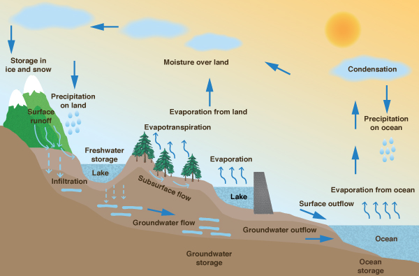
2.1 HYDROLOGY The hydrology studies the water on the Earth, from occurrence, circulation, distribution to chemical, physical and relation to living things. Hydrology encompasses surface and groundwater. The hydrological cycles are the recirculatory transport of water of the earth that is in the atmosphere, land, and oceans. The elements of the hydrological cycle are the atmosphere, vegetation, snowpack and icecaps, land surface, soil, streams, lakes and rivers, aquifers and oceans (Ponce, 1994). The liquid-transport phases of the hydrologic cycle are: precipitation from atmosphere onto land surface, through fall from vegetation onto land surface, melt from snow and ice to land surface, surface runoff from land surface to streams, lakes, and rivers, and from streams, lakes and rivers to oceans. Infiltration from land to surface soil, interflow from soil to streams lakes, and rivers and vice versa, percolation from soil to aquifers, capillary rise from aquifers to soil. Groundwater flow from streams, lakes and rivers to aquifers and vice versa and from aquifers to oceans and vice versa (Ponce, 1994). The vapor-transport phases of the hydrologic cycle are: (1) Evaporation from the land surface, streams, lakes, rivers, and oceans to atmosphere. (2) Evapotranspiration from vegetation to the atmosphere and vapor diffusion soil land and surface (Ponce, 1994). The U.S. Hydrology Department often uses the term watershed and basin to refers a catchment. Small catchment is called stream watershed, whereas large catchment is called river basin. The hydrology budget refers to an accounting of various transport phases of the hydrological cycle (Ponce, 1994).
2.2 CATCHMENT The catchment is part of the Earth's surface that collects runoff and concentrates it to release in downstream points. The runoff concentrated by catchment flows either into a large catchment or to the ocean (Ponce, 1994). The terms watersheds and basin are commonly used to refers to the catchment. Sometimes, the watershed is used to describe small catchment while the basin is used to describe large catchment. The interpretation of the hydrology cycle within the catchment's boundaries leads to the concept of hydrology budget. The hydrologic budget is the account of the all transport phases that occur in the hydrologic cycle. The following is a hydrologic budget equation for surface and groundwater (Ponce, 1994).
2.3 HYDROLOGIC MODEL Due to the constant degradation of the ecosystem, catchment models have been developed from traditional hydrological model to more precise and comprehensive to enhance the water management and maximize land productivity (Gericke and Du Plessis, 2012). Mathematical models have been developed to understand the complicated process that is happening in the hydrological process which has a direct link to geology, geomorphology, topography, weather, land use and human activities that must be analyzed and quantified (Ghoraba, 2015). Water, one of the elements of nature is primal for the survival of living things on the earth. Elements that govern the economics of countries is essential for developing the agriculture and industry. The ability of using and maintaining the water has become the core of nations developing strategies and regulations in regions (Ghoraba, 2015). Water balances have been used around the world to understand to study hydrologic effect under climate change scenarios. One of this model was developed by Thornthwaite and Mather (1957) by analyzing long-term monthly climate condition. Typical examples are (1) in South America a grid-based model by Vorosmarty el at, (1989); the Rhine flow model of Van Deursch and Kwadijk (1993) (Alemaw and Chaoka, 2003).
Figure 1. Water cycle 2.4 CONCEPTUAL MODEL The water cycle has three main components which are: precipitation, evapotranspiration, and runoff. Runoff is the amount of water that flows through the surface, the ground in the catchment. It is usually expressed in liter per second or millimeter per year. Therefore, runoff is the basic information related to water cycle showing how wet the catchment is. Runoff data is very variable during the years, and pressure over the water resources is variable over the year. These seasonal differences is a good indicator of water sensitivity during lowest monthly runoff expresses under water scarcity and drought (Frantar and Brancelj, 2013). Precipitation, snowfall and hail are part of the rainfall. Rainfall is used to describe precipitation. Generally, a catchment has an abstractive capability that acts to reduce total rainfall into effective rainfall. The differences between total rainfall and effective rainfall are the losses or hydrology abstraction. Its includes interception, infiltration, surface storage, evaporation, and evapotranspiration (Ponce, 2014). Discharge regime is an indicator of average river discharge fluctuations over periods (years). Multiple factors influence discharge regimes such as vegetation, climate, topography, bedrock, soil, and society. The primary factor is climate under precipitation, evapotranspiration, temperature, and snow cover duration (Frantar and Brancelj, 2013). The following formula is a hydrology budget equation for both surface and groundwater proposed by Ponce. (1994):
in which: ΔS = change in storage, P = Precipitation, E = Evaporation, T = Evapotranspiration, G = Groundwater outflow . Q = Surface runoff. A hydrological budget equation that considers only surface water is:
I = Infiltration. Within a given time span, under equilibrium conditions (ΔS = 0), equation 2 reduces to:
Equation (3) is imperfect due to it assumes that infiltration is lost from the surface water budget. It is returned to the control volume as evaporation from lakes and ponds, evapotranspiration or surface runoff (Poncea and Shetty, 1995). In the equation (3), the hydrology losses L are defined as the sum of evaporation, evapotranspiration, and infiltration:
Given the fundamental equation of flood hydrology:
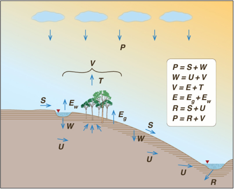
2.5 CYBERNETIC HYDROLOGY BALANCE Ponce and Shetty (1995) provide a background related to one of the fundamental problems in hydrology which is how much water could have a catchment over a defined period. The authors mentioned that there are: empirical models described by Rangeley (1960) and Ghoraba (2015); and continuous simulation models described by Crawford and Linsley (1966), and practical alternative models called conceptual model described by L'vovich's (1979). The conceptual model uses the hydrology budget in which the precipitation is divided into various components (Hamon, 1963). It divides annual precipitation into surface runoff, baseflow, and vaporization. The normal water balance applicable to the individual storm is:
The losses for an individual storm is the interception, surface storage, and infiltration. A water balance equation applicable on an annual basis is:
In which R is a runoff, including surface and subsurface runoff that includes (vegetated surface, non-vegetated surface and water bodies). Annual precipitation P can be separated into two components:
Then equation (8) includes more variables related to surface runoff and catchment wetting. The equation (8) is divided into two main components in which the catchment wetting consist of baseflow and vaporization. Wetting consists of two components :
Where U is baseflow, and V is the vaporization, the fraction of wetting returned to the atmosphere as water vapor. Vaporization, which comprises all moisture returned to the atmosphere, has two components:
Vaporization has two main components in which nonproductive evapotranspiration, hereafter referrers to as evaporation, and T = productive evaporation that is part of the transpiration from vegetated surface such as leaves and other parts of the plant use for their physiological needs, hereafter as evapotranspiration, In turn, evaporation has two components:
In which 1) Eg, evaporation from non-vegetated areas of Earth's surface and near-surface 2) Ew , evaporation from sizable water bodies such as reservoirs, lakes and rivers. Runoff (total runoff) is the sum of the surface and baseflow:
Combining equation 8, 9 and 12:
Equation 8 to 13 are set of water balance equations, combining equation 12 and 13 leads to:
Equation (14) separates annual precipitation of catchment into three major components (a) surface runoff, (b) baseflow, and (c) vaporization. Significantly, Eq 14 assumes that soil moisture year by year does not change; therefore it is negligible. Under L'vovich's hydrology budget, two water balance coefficients may be defined: (1) runoff coefficient, and (2) baseflow coefficient. The runoff coefficient is:
The baseflow coefficient is:
Therefore, the fundamental approach of cybernetic water balance is inductive and additive, that see the catchment as a whole system in which the runoff is equal to precipitation minus losses. It is characterized by the statement in which the precipitation is equal to runoff plus vaporization which help to know the yield hydrology. (Ponce and Shetty, 1995). The set of equations constitute L'vovich's water balance equations.
Figure 2. Elements of L'vovich's water balance
2.6 HORTON INDEX (HI) Horton Index is a dimensionless number between 0 to 1 that describes a fraction of a catchment wetting (Eq 9) uses in evaporation known as vaporation (Horton, 1933). HI is defined as:
According to Troch et al., (2009), HI provides a measure of vegetation water limitation in response to changes in precipitation. Voepel et al., (2011) demonstrates that HI values are signiicant high related both to climate and topographic characteristics. Thus, HI represents competition for W between plant water use (ET), and drainage to baseflow. Understanding how precipitation is partitioned into evapotranspiration, storage, and streamflow is a fundamental question in hydrology. From a catchment perspective, hydrologic partitioning is manifested in various spatial and temporal scales of a catchment. Runoff responses related to climatic forcing, catchment morphological, and pedological characteristics (Botter et al., 2007; Wagener et al., 2007).
2.7 GIS TECHNIQUE AND COMPUTER POWER Geographic Information System (GIS) and Remote Sensing (RS) are two fields that have been improved application of catchment models around the world. For example, GIS is a tool for managing many databases and proving visual representation of catchment's characteristics. Besides, catchment models using GIS improve them efficiently and increase the functionality of hydrologic models. (Alemaw and Chaoka, 2003; Ghoraba, 2015). GIS softwares have increased time-saving, results, analysis and data display for temporal and spatial digital hydrology data (Thomas). 2.8 GIS MODELS A model is a representation of essential aspects of the real world such as process, phenomenon, object, systems. Regarding GIS, it is a computer representation of spatial information. According to Longley, Goodchild et al, (2005) a computational model can be divided into two meanings: data model and spatial model. Data model. It is the representation of how the world looks likes in a digital data structure. After, this is used for GIS spatial analysis that could be represented as maps or spatial analysis to model some natural processes (Domnia, 2012). Spatial models. It is a spatial simulation model that shows natural, social, and economical process dynamically (, 2012). GIS techniques allow various analyzes of geographic elements of catchments that are part of landscapes (Frantar and Brancelj, 2013). All hydrologic models depend on the type of data available. It could be defined as internal variables and be constant (catchment geometry characteristics). The spatial model could be a spatial variable such as rainfall or meteorological parameters. 2.8.1 Types of spatial model Ackoff (1964), classified the spatial models in three principal areas:
Thomas and Hugget (1980), divided as you can see in the following Figure 3.
Figure 3.Classification of the models according to abstraction (Huggett 1980). On the other hand, Nir (1987) defined the following spatial model classification:
According to Domnia (2012), other factors can consider such as time, degree of the specification and how it is being used. Therefore, spatial model can be classified in:
There are two essential criterions to consider in hydrological model according to Beven (2003).
According to Serban (1995), there are two types of models which are: stochastic and deterministic models.
2.8.2 Reasons for spatial modeling
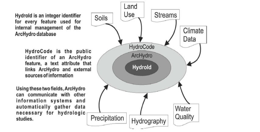
In addition to the above mentioned, there are other benefits to GIS automation for example, automation makes work easier, faster and work more accurate (Domnia, 2012). 2.9 HYDROLOGY MODELING DATA REPRESENTATION One of the most important hydrologic model available throughout ESRI is called ArcHydro developed at Center for Research in Water Resources in Texas by Maidment (2002). He considers that the main characteristics of the model is the structure (hydrological layers in GIS) and the application in water resources. 2.9.1 ArcHydro data model characteristics ArcHydro runs in ArcGIS , and it is composed in two parts. The first one, it is a geospatial and second one, it is a temporal model. ArcHydro has a spatial dataset that connects the features in it; also, it includes tools that allow manipulation and analyzation of hydrological data or creation of new spatial model. Arc Hydro uses a data structure for hydrology simulation models, but it does not contain any function to simulate hydrologic processes (Domnita, 2012). The modelling of hydrology process can be exchanged through data exchange, and independent hydrology model, through the model attached to Arc Hydro as a dynamic link library (dll) or through extending Arc Hydro objects. As a result, functions and data available can be used directly in ArcGIS or external programs calling library methods(Domnita, 2012). Another characteristic of Arc Hydro is that geospatial data can be combined, which stand for where hydrology process occurs in time. Arc Hydro was developed to use in water resources problems in any scale, and any specific modelling task. Arc Hydro consists of a set of layers that includes different terrains characteristics and structures to be modelled. Figure 5. The model information is stored in a series of simple data tables as part of feature classes, raster datasets, and attributes (Domnita, 2012). Water modeling can be applied for different purposes such as floods, water for supplied and quality, infrastructure design, landscape studies. Also, it requires to account for water behavior as well as water regulations that could be included in the model. ArcHydro creates object attributes to show the relationship between different elements from the same layer or other layers. As a result, ArcObjects uses ObjectId attribute to identify a feature in a feature class uniquely.
Figure 4. The ArcHydro identifiers and connections within the geodatabase 2.9.2 ArcHydro attributes ArcHydro has two attributes: HydroId and HydroCode. HydroId. It is an integer attribute that identified the feature inside the database, while the ObjectId uses in each feature can vary due to the spatial analysis or copying from one feature class to another. HydroId identifier relations between different features class can be made, and different types of hydrologic structures can be used in the same analysis. The management of the HydroId identifiers at database level has two tables, namely (LayerKeyTable and LayerIdTable which are created automatically). HydroCode. It is a text attribute standing for a public identifier of the feature. In other words, it is an external identifier for each element in a feature class and GIS manager can use the HydroCode to combine gauging station data to the feature class from the model, for example. 2.9.3 ArcHydro data model characteristics Digital elevation model (DEM) is a primary data structure for extraction and processing. It has a grid of cell, and every cell has a certain altitude value. Figure 5 is organized into five categories to show how Arc Hydro has organized: Flow elements, hydrography, flow network elements, flow channels, and time series (Zeiler, 2000).
Figure 5. Layers from ArcHydro Model
3 HYDROLOGIC CHARACTERISTICS OF CATCHMENTS
Essential characteristics of a catchment are: area, shape, relief, linear measures, topology, density, and drainage patterns. 3.1 CATCHMENT AREA It is perhaps the most crucial characteristics because it determines the potential runoff volume, provided the storm covers the whole area. The topographic measure is most reliable that the hydrologic divide for practical use. The topographic divide is delineated on a quadrangle sheet. The direction of surface runoff is perpendicular to the contour line. All peaks and saddle are identified at the outset. The runoff in the peak runs in all direction while the runoff in the saddle is in the two opposite directions perpendicular to the saddle axis (Ponce, 1994). Several formulas have been proposed. One of them is the following:
Qp = Peak flow A = Area of the catchment c and n = Parameter defined the regression analysis. 3.2 CATCHMENT SHAPE The catchment shape is the outline described by the horizontal projection of a catchment. The following formula describes it:
A = Catchment area L = Catchment length, measure along the longest watercourse. Area and length are given in square kilometers and kilometers. There is another parameter that derived from the catchment perimeter that is compactness ratio. It is the ratio of the catchment perimeter that the equivalent circle. The following formula describes it:
Kc = Compactness ratio P = Perimeter of catchment A = Catchment area Compactness ratio close to 1 describes a catchment having a fast and peaked catchment response. On the other hand, compactness ratio larger than 1 describes a catchment with a delayed runoff response. However, other elements that are part of the catchment should be considered such as catchment relief, vegetation, drainage density (Ponce, 2014). 3.3 CATCHMENT RELIEF Relief is the differences between two references points. Maximum catchment relief is the elevation difference between the highest point in the catchment divide and the catchment outlet. The mainstream is the central and largest watercourse of the catchment and the one conveying the runoff to the outlet the relief. The hypsometric analysis describes the overall relief of catchments. The hypsometric curve is used when a hydrologic variable such as precipitation, vegetation cover or snowfall shows differences according to altitude. The relief ratio helps to measure the intensity of the erosional process active in the catchment (Ponce, 2014).
3.4 LINEAR MEASURES These are used to describe the one-dimensional feature of the catchment. The hydraulic length (L) is the length measured along the principal watercourse (Ponce, 2014). 3.5 BASIN TOPOLOGY Basin topology refers to the regional anatomy of the stream network. Distributed rainfall-runoff modeling needs the hierarchical description of stream connectivity of its topology. Therefore, the stream order classified streams in hierarchical numerical order from zero order which is the overland flow, then the first order stream that received from the zero order. Two first order stream combined to form a second-order stream. Large catchment could have stream orders of 10 or more (Ponce, 2014). Catchment geomorphology plays a role in the relationship between vegetation cover, landscape evolution and water status (Rasmusses at al 2010). In semiarid basins, differences in vegetation between the north and south facing slopes in association with different soil moisture states (catchment wetting) posed a dominant control over the geomorphology of the basin (Yetemen et al., 2010). The two main parameters from geomorphology of a catchment are: slope and elevation that control the annual precipitation, and these two parameters can be retained long enough in a catchment for the available vegetation (Voepel et al., 2011). 3.6 DRAINAGE DENSITY Drainage density is the ratio of the total stream length (the sum of the length of the streams) to the catchment area. High density indicates fast and peaked runoff response, whereas low density reflects delayed runoff response (Ponce, 2014). 3.7 Drainage patterns Drainage patterns in catchments vary widely. The more intricate patterns are the result of high drainage density, and they reflect geology, soil, and vegetation effects. Drainage patterns are often related to hydrological properties such as runoff response or annual water yield. The most common drainage patterns are dendritic, rectangular, radial and trellis (Ponce, 2014). The catchment area and its physical analysis will use GIS and data analysis tool for hydrology. This data could be but exclusive to following parameters (drainage area, perimeter, catchment hydraulic length, form ratio, compactness ratio, maximum elevation, minimum elevation, average land surface slope, stream slope, total channel length, drainage density) (Gericke and Du Plessis, 2012). Analysis model of a catchment is essential for two reasons. First, it helps to delineate the catchment boundaries and corresponding discharge point. Secondly, it helps to understand surface runoff processes. Also using GIS, models help to determine suitable location and volume of reservoirs for yield hydrological budget (Barnalin and Venkatesh, 2016). The evolution of landscape models confirm the dominant role of vegetation in climates limited by water (Collins and Bras, 2010; Istanbulluoglu and Bras, 2005), It suggests that response of vegetation to climatic gradients affects the density of drainage, relief, and concavity of channels, which reproduces empirical patterns in the density of drainage with climate (Abrahams and Ponczynski, 1984). Rasmussen et al., (2011) used catchment data from different climates and common lithology to demonstrate that energy and mass flow associated with primary production. Effective precipitation explains substantial variation in the structure, and functions of the catchment.
4 DESCRIPTION OF ECOSYSTEM IN CALIFORNIA
California is a house of diverse ecosystem and biota, covering more than 150,000 square miles. Its territory has mountains, valleys, coasts, and desert. It gives different climate conditions around it. From east to west there is the Sierra Nevada region, coastal mountain ranges to the Pacific Ocean (US EPA, 2012). California's water quality management has defined eight ecological regions: North Coast, Central Valley, Coast and interior Chaparral, South Coast, West Sierra, and Central Lahontan, Desert-Modoc. (Group, n.d.)
Figure 6. Water ecosystems in California. The San Francisco Bay-Delta watershed's extension is 75,000 square miles. For the north, the watershed extends to 500 miles to the Cascade Range in the north to the Tehachapi Mountains. For the south and east, it is bounded by Sierra mountain, and for the west to the Coast Range. According to the United States Environmental Protection Agency: "The San Francisco Bay-Delta provides water to 25 million Californians, irrigation for 7000 square miles of agriculture, and includes important economic resources such as California's water supply infrastructure, port, deep-water shipping channels, major highway and railroad corridors and energy lines" (California Department of Water, 2003a)
4.1 THE NORTH AND COAST HYDROLOGY REGIIONS The North region covers approximately 14,470 square miles including Modoc, Siskiyou, Del Norte, Trinity, Humboldt, Mendocino, Lake and Sonoma counties. In 1995 the population was 606,000 inhabitants with most of them live in center along the Pacific coast and in the inland valleys north of the San Francisco Bay Area. The rural area is extended for the northern mountainous portion of the region. The land is covered heavily with forest. There are irrigation areas along to the narrow river valleys. The main crops are alfalfa, grain and pasture, In the south portion of the Coast hydrological region the main crops close to the urban areas are wine grapes, nursery, stock, orchards and truck crops (California Department of Water, 2003b)
Figure 7. Water storage and distribution California. The South Coast Region covers approximately 10,600 square miles of the South California catchment that drains to the Pacific Ocean. Between the most important and significant geographic feature are: The coastal plain, The central Transverse Range the Peninsular Ranges and the San Fernando, San Gabriel and Santa Ana River and Santa Clara Rivers valleys (California Department of Water, 2003b). 17 million people are living within the boundaries of South Coast Hydrologic Region which represents 50% of California's population located over Metropolitan areas surrounding Ventura, Los Angeles, San Diego, San Bernandino, and Riverside (California Department of Water, 2003a).
4.2 CALIFORNIA PRECIPITATION
Figure 8. California's average precipitation from 1990 to 1960. The precipitation behavior is variable year by year and trying to understand this behavior is critical for water management and policy. The California climate is the Mediterranean; cold, wet winters and warm and dry summers. From October to April are cold season and precipitation falls. In the state, southeast areas can receive less than 5 inches while in the north coast areas could receive 100 inches in a year. The average precipitation according to the Northern California 8 station from the California Department of Water resources is 50 inches per year. Given the sense of how much the Sacramento River catchment received it, which the most important water supply in California (CA State Climatologist, 2017).
To apply the cybernetic hydrological model using the California catchment data, I will use the geographical and rainfall-runoff data available online through the California states websites (NOAA, 2018). Digital elevation models will be used from the USGS virtual platform (Earth Explore) and (Alaska Satellite Facilities). Precipitation data are available in the National Centers of Environmental Information (NOAA, 2018). 5.1 STUDY AREA
5.1.1 Russian River catchments near Guerneville, California
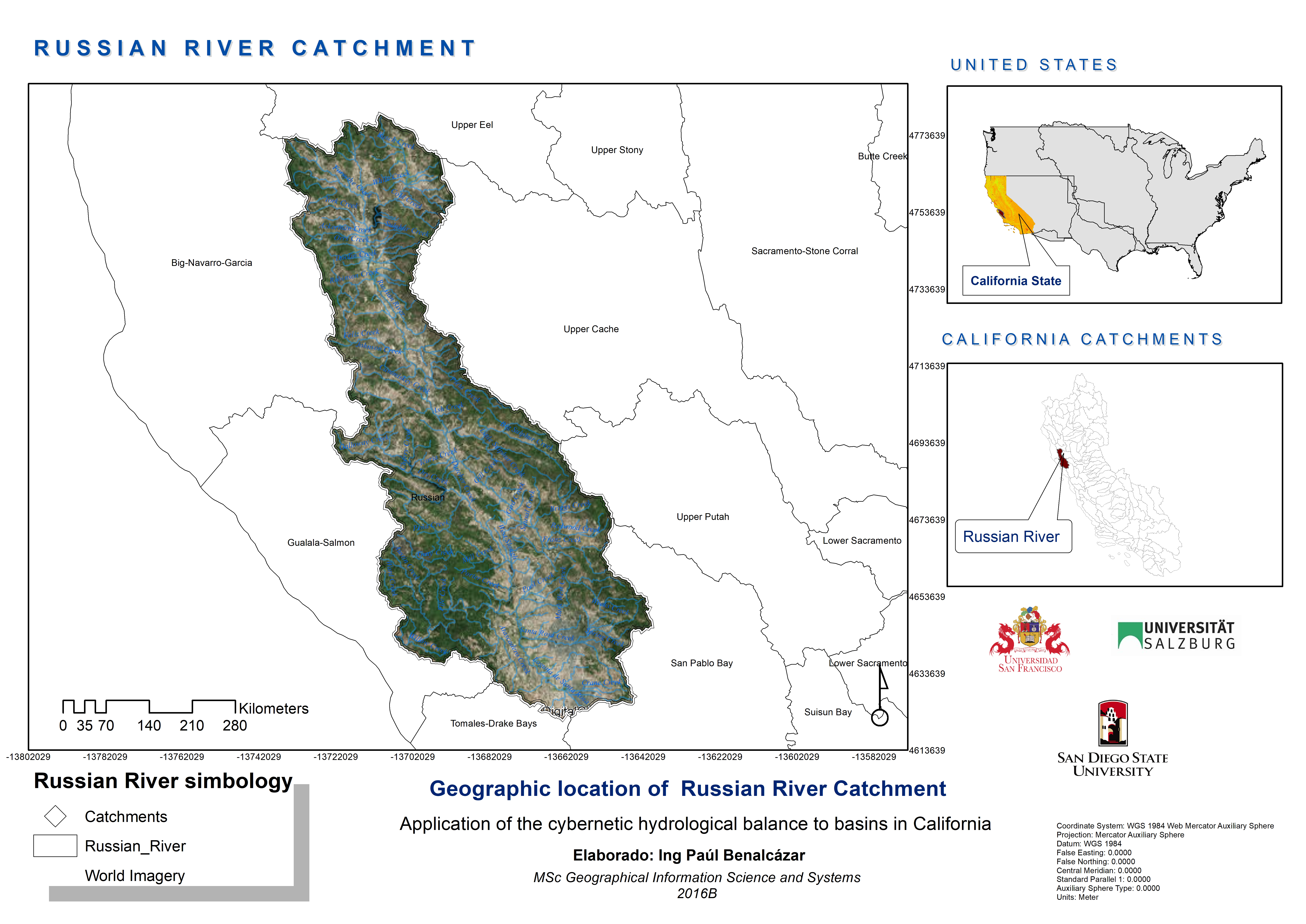
Figure 9. Russian River geographic location. The Russian River Catchment has 1,500 square miles of agricultural, forest and urban area in the northern Sonoma County and southern Mendocino County California. People supply their demands using surface and groundwater for irrigation, municipal and private and industrial-commercial uses. In the agricultural part, they uses for winery and also for recreation (USGS, 2018a). The Russian River is prone to droughts due to the hydrological variation responding to extreme climate variation plus increasing water demands which is a challenge for environmental and water resources managers to ensure that it would not have depletion.
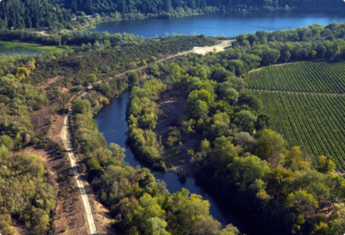
Figure 10. Russian River Valley (USGS, 2018). 5.1.2 Salinas River catchment, Spreckles, California
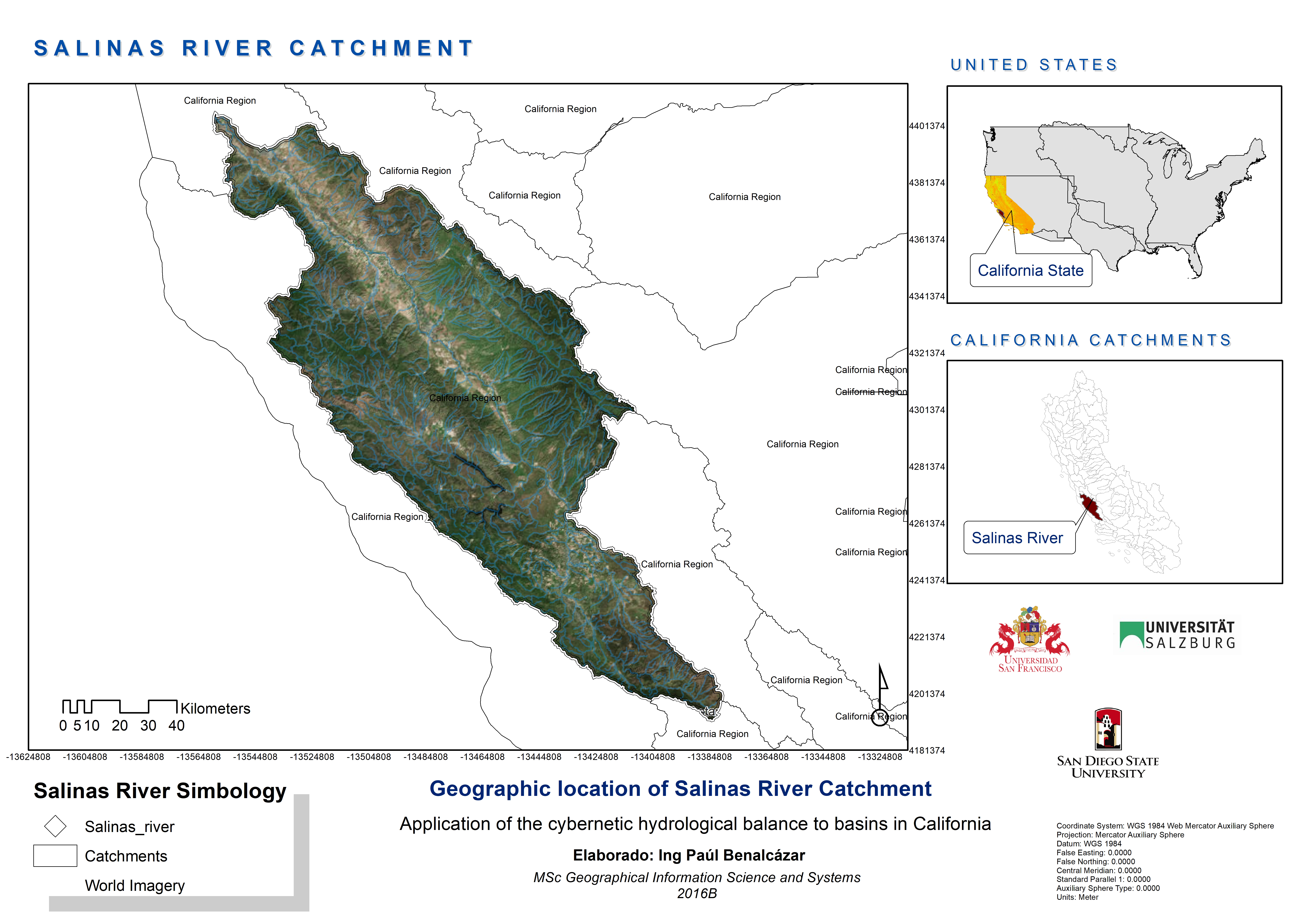
Figure 11. Geographic location of Salinas River. The Salinas river is part of the riparian corridor in the Central Coast of California. It has 4,600 square miles of land in the Monterrey and San Obispo Counties. The catchment includes 200,000 acres of irrigated agriculture, fish and wildlife habitat. Urban expansion, agricultural runoff have been affected the wildlife, native fish and water quality in these catchment (Central Coast Regional Water Quality Control Board, 2017).
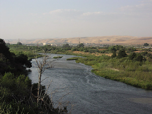
Figure 12.Salinas River in the foreground (Central Coast Regional Water Quality Control Board, 2017.
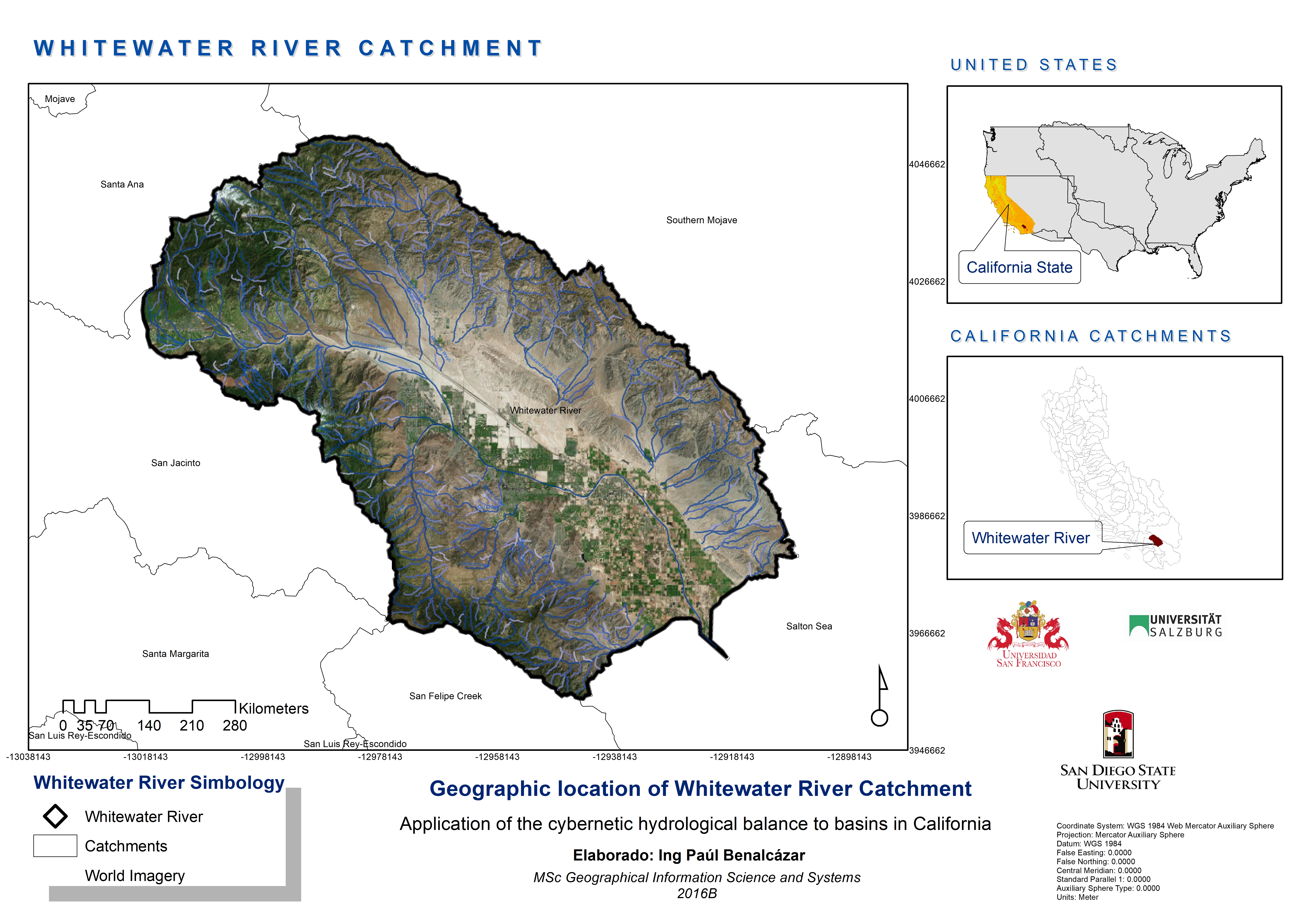
5.1.3 Whitewater River catchment near Mecca, California
Figure 13. Geographic location Whitewater River. The Whitewater river is a small permanent stream in western Riverside County, California, with small upstream section in southwestern San Bernardino county. It is located close to San Gregorio Mountain, San Bernandino Mountains and San Bernandino County. Before Palm Spring, the Whitewater river is fed imported water from the Colorado River aqueduct by the Metropolitan Water District of Southern California (Whitewater River-California, 2017).
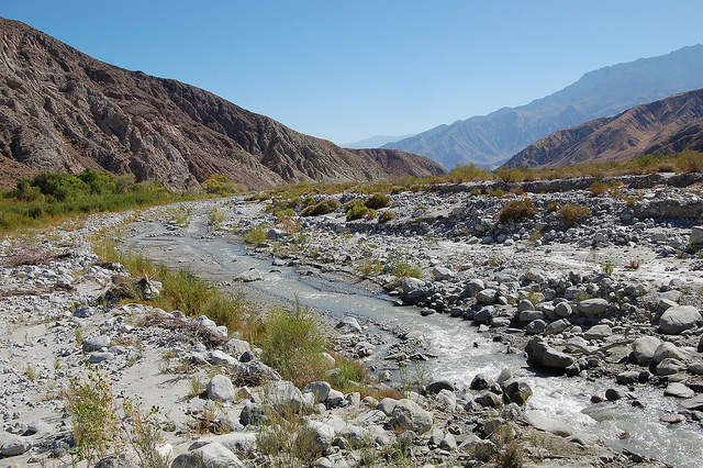
Figure 14.Whitewater River Whitewater Canyon (Whitewater River, California 2017).
5.2 CYBERNETIC HYDROLOGIC BALANCE MODEL The following equations were used to formulate the hydrologic model using L'vovich's model. Equations 8 to 12 were applied. Discharge and precipitation are in millimetres (Ponce and Shetty, 1995). The following steps were applied:
After applied the above steps P, R, S, U, W, and V hydrologic values were obtained for the overall indicator of the catchments. 5.3 GIS APPLICATION The DEM of catchment were obtained using the Earthexplore.usgs.gov website services from USGS platform of the NASA LPDSSC Collection-Aster Collections-ASTER global (Ariza, 2013). It was extracted, projected and transformed for each catchment of the study area. Specific GIS data features such as line, polygons, and points were extracted and created using the Clip and Extract analysis toolbox. Before starting to run the Arc Hydro packages, the DEM needed a pre-conditioning hydrology process. Maidment (2002) describes that the pre-conditioning process is known as the Anedum (Topo to Raster). The preconditioning process is used to reduce the possible errors in digital elevation models like sinks in areas of low elevation. To correct it, the Topo to Raster tool in ArcMap was used. The DEM was prepared, and it was converted to points using the raster to points tool, then adding to contour, breakpoint-streams (called streams), and boundaries were added to the Topo to Raster tool (Table 2). After that, the new DEM was obtained.
The output cell was 15 m as the original DEM. In the environment tab/ processing extent, the DEM was used in Snap Raster. Catchment polygons were used to cut out pieces of feature class as a cookie cutter. (Gericke and Du Plessis, 2012) Data extraction was followed by transformation, attribute table editions and calculation of the catchment geometry (areas, perimeters, and distances). After that, Venkatesh. (2012), describes the process to obtain watershed and stream network delineation using Arc Hydro tools.
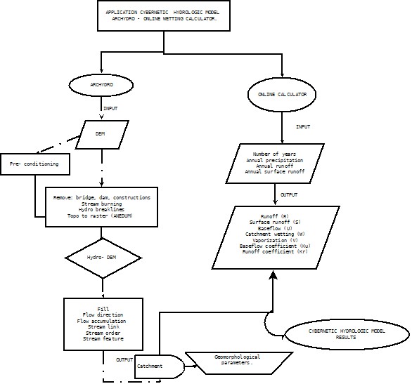
5.3 APPLICATION OF THE CYBERNETIC HYDROLOGIC MODEL DIAGRAM
Figure 15. Cybernetic Hydrology Model Scheme. 6. RESULTS AND ANALYSIS
6.1 RESULTS 6.1.1 Data sources of Russian River near Guerneville, California
6.1.2 Data sources of Salinas River, California
6.1.3 Data sources of Whitewater River, California 6.1.3 Data sources of Whitewater River, California
6.2 ANALYSIS OF THE BASEFLOW AND RUNOFF COEFFICIENT TO EACH CATCHMENT 6.2.1 Russian River
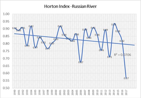
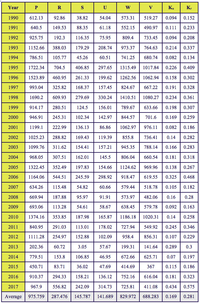
Descriptive statistics were used to analyze 28 years of diary precipitations and discharge data from 1990-2017. Precipitation, discharge, surface runoff, base flow, catchment wetting, vaporation, base flow coefficient, and runoff coefficient where obtained using the catchment wetting online calculator (see Table 15) for the Russian River catchment. 6.2.2 Horton Index Russian River
Figure 17. Russian River Horton Index from 1990 to 2017. According to the climatic spectrum in subtropical regions, published in Ponce, (2012), The Russian River is located in a Sub humid region (average P = 975.76 mm ( SD = 350.28). (Table 6). The mean catchment wetting is 829.97 mm (SD 51.79 mm). The average Horton Index was 0.82; indicating that 82% of catchment wetting (W) was used as vaporation ;known as evapotranspiration. Figure 17. The Cv of P = 0.37 which is the interannual variability of precipitation that leads to more drough0t (Steinscheneider, 2018). The vaporation was 688.28 mm from 1990-2017 being similar to Flint et al., (2013) as part of the potential evapotranspiration for water years 1981-2010, calculated by the Basin characterization model for California. It is important to notice that S and U are almost similar (SD >85), corresponding to a sub-humid region of the catchment. 6.2.3 Salinas River
Descriptive statistics were used to analyze 28 years of diary precipitations and discharge data from 1990-2017. Precipitation, discharge, surface runoff, base flow, catchment wetting, vaporation, base flow coefficient, and runoff coefficient where obtained using the catchment wetting online calculator (see Table 15) for the Russian River catchment. 6.2.4 Horton Index Salinas River
Figure 18. Salinas River Horton Index from 1990 to 2017. According to the climatic spectrum in subtropical regions, published in Ponce, (2012), The Russian River is located in a Sub humid region (average P = 975.76 mm ( SD = 350.28). (Table 6). The mean catchment wetting is 829.97 mm (SD 51.79 mm). The average Horton Index was 0.82; indicating that 82% of catchment wetting (W) was used as vaporation (known as evapotranspiration) Figure 17. The Cv of P = 0.37 which is the interannual variability of precipitation that leads to more drough0t (Steinscheneider, 2018). The vaporation was 688.28 mm from 1990-2017 being similar to Flint et al., (2013) as part of the potential evapotranspiration for water years 1981-2010, calculated by the Basin characterization model for California. It is important to notice that S and U are almost similar (SD >85), corresponding to a sub-humid region of the catchment. 6.2.5 Whitewater River
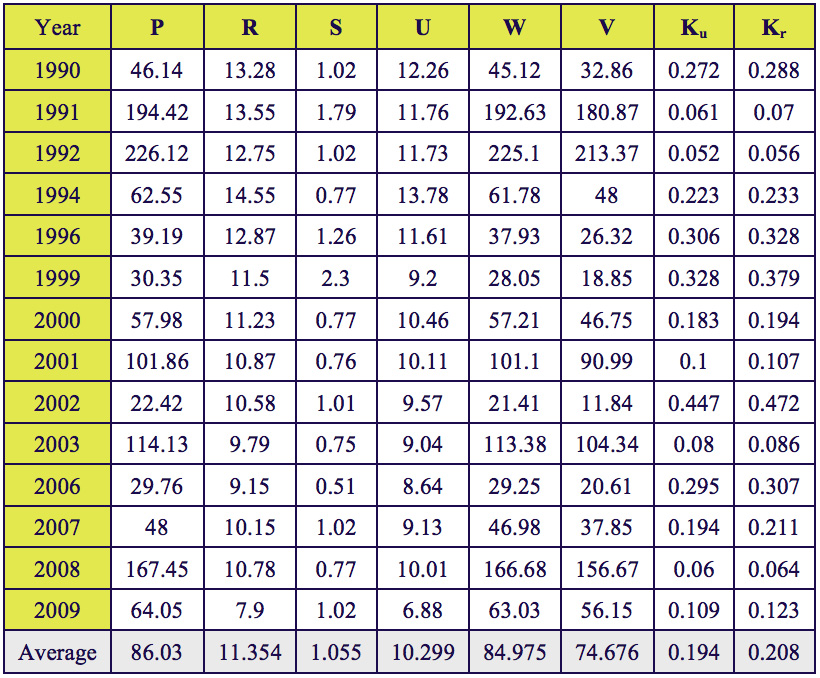
Descriptive statistics were analyzed using 24 years of diary precipitations and discharge data from 1993-2013 and 2017, in which precipitation, discharge, surface runoff, base flow, catchment wetting, vaporation, base flow coefficient, and runoff coefficient where obtained using the catchment wetting online calculator (Table 16) for Salinas River catchment. 6.2.6 Horton Index Salinas River
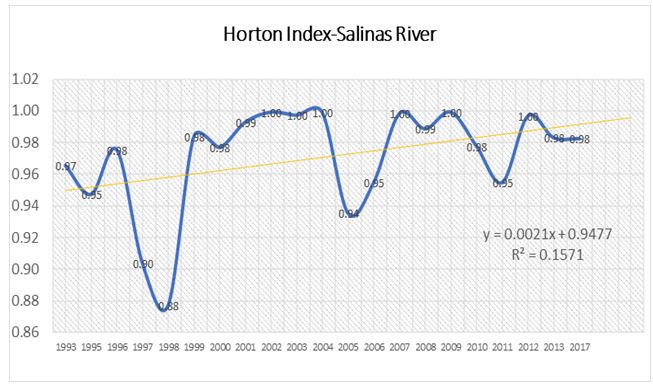
Figure 19. Salinas River Horton Index from 1993 to 2017. According to the climatic spectrum in subtropical regions, published in Ponce, (2012). Salinas River is located in Arid region (average P= 366.19 mm), SD of 135.90 (Salinas River Table 7). The mean catchment wetting is 352.04 mm (SD 25.37 mm). The average Horton Index was 0.97, indicating that 97 % of the catchment wetting is used to evapotranspiration (Figure 18). The Cv of P= 0.36 which is the interannual variability of precipitation that leads to more drought (Steinscheneider, 2018). The vaporation was 339.98 mm from 1993-2013 and 2017 which is similar to Flint et al., (2013) as part of the potential evapotranspiration for water years 1981-2010, calculated by the Basin Characterization model for California. The amount of surface and base flow to the arid region is 14.15 mm (SD = 15.58) and 12.06 mm (SD= 15.76); as a result, there is not much variation. The surface runoff is negligible to this area.
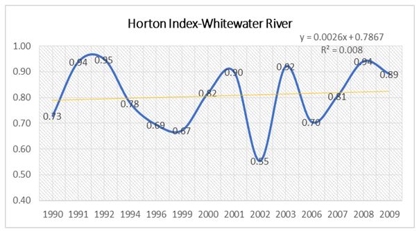
6.3 ANALYSIS OF PRECIPITATION, RUNOFF AND BASEFLOW FOR THE CATCHMENTS 6.3.1 Precipitation Precipitation across California's catchment was variable (Table 15, Table 16, Table 17) during the periods 1990-2017. Rainfall variations were associated with the phenomenon called Atmospheric River floods (AR), which contributed between 20-50% of the state's precipitation and streamflow (Dettinger et al., 2011). Year by year the variability shows a coefficient of variation (Cv) higher than 0.35 for all catchments. This Cv was higher in the Whitewater River Cv= 1.04(Table 17). Floods of the Russian River in 1998 and 2010 were associated directly to AR floods in central California (Dettinger et al., 2011). 6.3.2 Base flow coefficient Due to climate spectrum of the two catchments (Salinas River (arid region), and Whitewater River (super arid region), base flow is an essential element of the groundwater available (98% of groundwater appears as base flow) (Ponce, 2012). Its reduction could cause drying up of spring and wetlands areas, the die-off of riparian vegetation, and the reduction of base flow in nearby streams. In these two catchments, the mean U are 12.06 (SD= 3.44) and 10.30 (SD=2.38) respectively, so base flow is a crucial water supply in these regions. On the contrary, the Russian River had an average U= 141.69 (SD=85.24) where the surface runoff is the main water supplied; then base flow is the second water supplied for the region (USGS, 2018). 6.3.3 Runoff coefficient In arid region (Salinas River and Whitewater River) climatic spectrum is less than 300 mm of mean annual precipitation, the surface water is little (scarce runoff). The runoff coefficient is 10-15% of the precipitation. In the humid region (Russian River), the middle of the climatic spectrum is 800 mm of mean annual precipitation, about 39% of the precipitation is part of streamflow (runoff). Values that agree with previous studies conducted by Lʹvovich, (1979); and Ponce, (2012). 6.3.4 Horton Index There are consistent patterns found in the two arid catchments. Driest areas and driest year exhibited both higher and less variable Horton Index (Table 16, and Table 17) whereas the humid catchment (Table 16) had less Horton index value. (Horton, 1933; Voepel et al., 2011). The HI increase as a catchment becomes drier and become closer to HI =1 in drier regions and during dry years (Sivapalan et al., 2011). The Horton Index observed during the periods of study 1990-2017 shows a direct correlation between the climate spectrum in subtropical regions and the HI. Horton index values match to arid and sup arid regions were the HI = 1 for most of the years. On the other hand, the sub-humid region was HI = 0.52 due to the northern location in the California county. That information shows the general pattern due to climate change in which arid region will become driest, and wet areas will become wettest as the information indicates (Cayan et al., 2008). Climate change has been affected by snow catchment hydrology (Gleick, 1987) as it part of the Russian River where the temperature has increased, and snow decreased (Cayan et al., 2008). The timing of snowmelt stressing water managers for water supplies or flooding events through annual precipitation (Huntington and Niswonger, 2012). The ability to predict the water balance in a catchment depends on different factors such as climate spatial-temporal variability (by looking to GIS and Remote sensing techniques), calibration of parameters to catchment models, and determination of variability and distribution of vegetation (Xu et al., 2012). The study shows that Russian River located in Northwest of California is primary wet with significant values of Kr and Ku, whereas arid zone (Salinas River) and super arid (Whitewater River) located in the Southernmost quarter of California are prevailing dry with negligible runoff and few wet years as Moran, (2017) found on his work. Although analyzing three catchments in California states is not statistical significance, the analysis of periods from 1990 to 2017 showed a reduction of HI into arid regions and HI increases in trends in semi-humid regions. Climate change poses a significant effort to predict water balance to regions, but it is essential to take into account that indirect impacts could be more significant than direct effects (Jones, 2011).
6.4 ARCHYDRO GEOMORPHOLOGICAL MODEL Catchment area and its physical analysis were obtained using Arc Hydro and data analysis tool for hydrology. The following parameters were obtained: drainage area, perimeter, catchment hydraulic length, form ratio, compactness ratio, maximum elevation, minimum elevation, average land surface slope, stream slope, total channel length, and drainage density (Gericke and Du Plessis, 2012). The following geomorphological characteristics for each catchment of California are described here:
6.4.1 Russian River
6.4.2 Salinas River
The catchment is located between 6 to 1783 mls. Its drainage area is 13167 km2, and its average land surface slope is 26.21 m/m with form ratio of 0.18, and compactness ratio (kc) of 0.04. 6.4.3 Whitewaters River
The catchment is located between - 69 to 3490 mls. Its drainage area is 3884.18 km2, and its average land surface slope is 0.26 m/m with form ratio of 0.24 and compactness ratio (kc) of 2.10.
6.5 CYBERNETIC HYDROLOGY MODEL MAPS-GIS APPLICATION Using values of Ku and Kr from the online calculator, a table of attributes were built in ArcMap to analyze runoff and baseflow for each catchment temporally. 6.5.1 Russian River baseflow coefficient
Figure 21. Russian River baseflow coefficient. Multitemporal analysis of the Russian River baseflow coefficient from 1990, 1994,1998,2002,2006,2010,2014 and 2017 was portrayed. In 2006 and 2017 the baseflow coefficient shows high values, which means that more baseflow water was available to those years for the region (Figure 20). It was due to precipitation conditions available to the same year and the geomorphology of the catchment (Ku = 0.32-0.43). On the other hand, during the 1990 and 1994, baseflow coefficient showed the worst scenarios in which Ku was between 0.09 to 0.07 (Table 15). 6.5.2 Russian River runoff coeficient
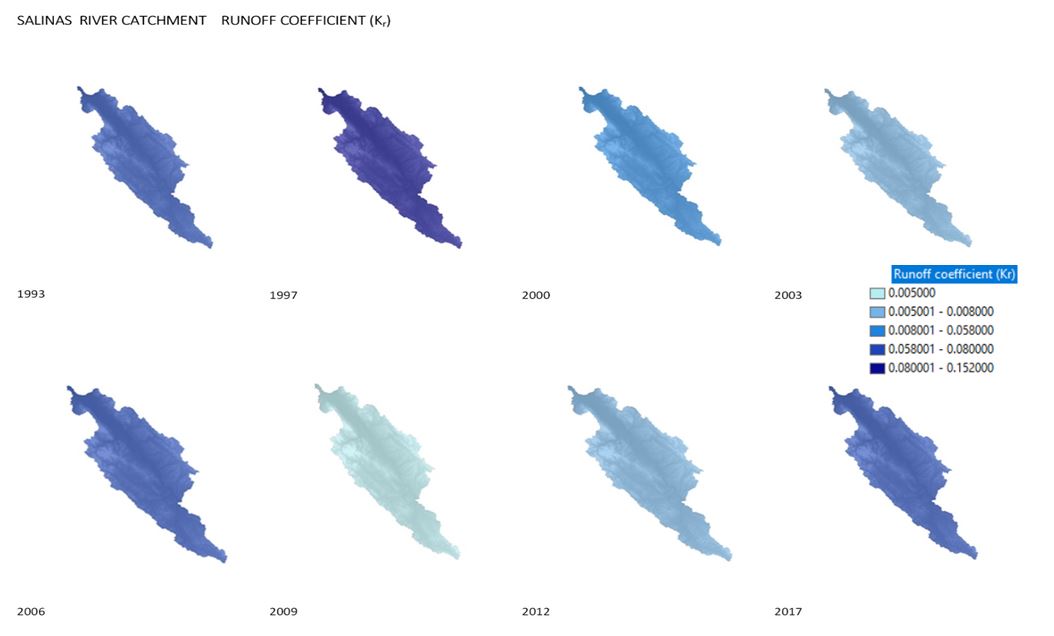
Figure 22. Russian River runoff coefficient. In figure 22, there are two main years where Kr coefficient is 0.36-0.57, which means that those years were wet. On the other hand, 1990, 1994 were dried. Years 1998, 2002, 2010, 2017 show Kr coefficient values between 0.28 to 0.15. 6.5.3 Salinas River baseflow coefficient
Figure 23. Salinas River baseflow coefficient.
Multitemporal analysis over Salinas River shows different baseflow coefficient
due to climate conditions, and geomorphology of the catchment. In 1999 had the
highest Ku coefficient available to the catchment 6.5.4 Salinas River runoff coefficient
Figure 24. Salinas River runoff coefficient. The figure 24 shows in 1993, 1997, 2006, and 2017 values of Kr = 0.08 to 0.15. Those values did not represent a problem for flood because of the amount of surface runoff available for that year, and Kr is not high enough to cause problems to infrastructure (The California Water Boards, 2011). For the other years, the runoff coefficient values were less than 0.005, showing that the Salinas River is an arid region, and there is not enough runoff water available that could have an economic worth. 6.5.5 Whitewater River runoff coeficient
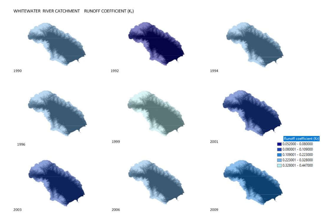
Figure 25. Whitewater River baseflow coefficient. Multitemporal analysis of the Whitewater river baseflow coefficient from 1996 to 2009 shows different behaviours due to climate conditions, and geomorphology of the catchment. There were four essential periods in which Ku = 0.22-0.32. Baseflow as part of the groundwater denoted a valuable resource for communities around the Whitewater River. In contrast, during 1992, 2003 were less than Kr = 0.05 as a result of climate conditions variability (Knowles Noah and Cayan Daniel R., 2002). 6.5.6 Whitewater River baseflow coeficient
Figure 26. Whitewater River runoff coefficient.
During the period of 1999, figure 26 shows that the Whitewater River had high values of Kr = 0.32 to 0.44, but during the rest of periods, especially 1992, 2011, and 2003, these Kr values were less than 0.1; indicating that the Whitewater River is a Super Arid region where runoff doesn't exist and baseflow is the primary sources of groundwater (Ponce, 2012). 7 CONCLUSIONS AND RECOMMENDATIONS
7.1 CONCLUSIONS The fundamental approach of cybernetic water balance is inductive and additive. It means that catchment can be seen as a whole system in which runoff is equal to precipitation minus losses, and it is equal to runoff plus vaporization. The cybernetic hydrology model is a model used since 1979, and it has been applied for water balance using the concept of the wetting catchment. Vegetation and water availability are considered to define how much surface flow and baseflow a catchment has by looking at the water pressure to surface storage and groundwater resources. This model has been applied in the region to estimate distribution runoff (fresh water) and shown the potential of water deficits to California catchments. The cybernetic hydrologic model developed by L'vovich's 1979 and Ponce and Shettle 1995 incorporate water budget analysis, which is divided into two main components. 1) Highly interconnected nature of a catchment associated with a geomorphological characteristic of a catchment. 2) Spatial and temporal representation of water balances of catchment helps water managers to understand what the current behaviour of the area is. Also, by adding the GIS and RS technology not only the geomorphological characteristics can be studied but also the ecological, pedological and anthropological process in the multiscale variability could be done. The cybernetic hydrology model helps to predict regional patterns of mean annual water balance, as well as interannual variability in individual catchments. The analysis shows that there is close symmetry between spatial variability of mean annual balance and general trends of temporal variability in individual catchments. Consequently, the cybernetic hydrology model provides an excellent framework to evaluate not only how the plant responds to water availability but also how this water availability is linked to the geomorphology of a catchment described by geomorphological GIS analysis. The application and incorporation of GIS technology (ArcHydro) have proven to be a significant advance in hydrology science not only for preprocessing but also for post-processing Results, analysis and visualization of hydrology models. Also, features such as Kr and Ku may change over time because of adding new contributing factors or geospatial analysis that can support new studies for the cybernetic hydrology model. Thanks to GIS and RS techniques, new phenomena has observed on the Earth such (Atmospheric River impacting California state), and its influences in the water balance budget. The amount of water available to vegetation (HI) is quantified using spatial and temporal GIS analysis tools. As a result, a new body of knowledge related to GIS-and Eco-hydrology has developed for further studies. The scale of information needed for water managers is often beyond numbers and statistical results, as the catchment wetting online calculator had shown. The fusion between online calculator and Arc-Hydro tools and its functionality integrate spatial, temporal, and statistical analysis for the catchments so that managers and policymakers can see, analyze, and take decision geo-spatially for water availability in the three catchments under the study. Runoff and baseflow values are complex mechanisms affected by precipitation and its distribution in time and space. Two parameters are linked to the geomorphology (drainage, hillslope, land use, soil infiltration rate, snow cover, vegetation, and human intervention), which significant; and they need to be considered for better water yield results. 7.2 RECOMMENDATIONS The cybernetic hydrologic model can be applied in areas like Ecuador due to the few data requirements for the model (precipitation and discharge). Weather information that could be compiled using local information for a catchment or satellite, plus adding remote sensing and GIS tools.
8. REFERENCES
9. ANNEXES 9.2 RESULT OF ONLINE CALCULATOR FOR U, W, V Ku, U, AND K r
Table 15. Ku and Kr of Russian River.
Table 16. Ku and Kr of Salinas River.
Table 17. Ku and Kr of Whitewater River.
| ||||||||||||||||||||||||||||||||||||||||||||||||||||||||||||||||||||||||||||||||||||||||||||||||||||||||||||||||||||||||||||||||||||||||||||||||||||||||||||||||||||||||||||||||||||||||||||||||||||||||||||||||||||||||||||||||||||||||||||||||||||||||||||||||||||||||||||||||||||||||||||||||||||||||||||||||||||||||||||||||||||||||||||||||||||||||||||||||||||||||||||||||||||||||||||||||||||||||||||||||||||||||||||||||||||||||||||||||||||||||||||||||||||||||||||||||||||||||||||||||||||||||||||||||||||||||||||||||||||||||||||||||||||||||||||||||||||||||||||||||||||||||||||||||||||||||||||||||||||||||||||||||||||||||||||||||||||||||||||||||||||||||||||||||||||||||||||||||||||||||||||||||||||||||||||||||||||||||||||||||||||||